5 Steps to Build Beautiful Stacked Area Charts with Python

---

---

Motivation

Telling a compelling story with data gets way easier when the charts supporting this very story are clear, self-explanatory and visually pleasing to the audience.

In many cases, substance and form are just equally important. Great data poorly presented will not catch the attention it deserves while poor data presented in a slick way will easily be discredited.

I hope this will resonate with many Data Analysts, or anyone who had to present a chart in front an audience once in their lifetime.

Matplotlib makes it quick and easy to plot data with off-the-shelf functions but the fine tuning steps take more effort. I spent quite some time researching best practices to build compelling charts with Matplotlib, so you don't have to.

In this article I focus on stacked area charts and explain how I stitched together the bits of knowledge I found here and there to go from this…

… to that:

All images, unless otherwise noted, are by the author.

---

0 The Data

To illustrate the methodology, I used a public dataset containing details about how the US are producing their electricity and which can be found here – https://ourworldindata.org/electricity-mix.

On top of being a great dataset to illustrate stacked area charts, I also found it very insightful.

Source: Ember – Yearly Electricity Data (2023); Ember – European Electricity Review (2022); Energy Institute – Statistical Review of World Energy (2023) License URL: https://creativecommons.org/licenses/by/4.0/License Type: CC BY-4.0

After importing the necessary packages to read the data and build our graphs, a few simple data transformation steps are required to get to the desired format:

1. Read the data
2. Filter on US figures only
3. Rename the columns for easier handling
4. Convert the ‘Year' column to the right datetime format
5. Set the ‘Year' column as index

import pandas as pd
import Matplotlib.pyplot as plt
from matplotlib.ticker import MaxNLocator, MultipleLocator
from matplotlib.dates import YearLocator, DateFormatter

# Read the data
df = pd.read_csv('electricity-prod-source-stacked.csv', sep=',')

# Keep only the data related to the US
df = df[df['Entity'] == 'United States']

# Rename the columns
df.rename(columns={'Other renewables excluding bioenergy - TWh (adapted for visualization of chart electricity-prod-source-stacked)': 'Other renewables',
                   'Electricity from bioenergy - TWh (adapted for visualization of chart electricity-prod-source-stacked)': 'Bioenergy',
                   'Electricity from solar - TWh (adapted for visualization of chart electricity-prod-source-stacked)': 'Solar',
                   'Electricity from wind - TWh (adapted for visualization of chart electricity-prod-source-stacked)': 'Wind',
                   'Electricity from hydro - TWh (adapted for visualization of chart electricity-prod-source-stacked)': 'Hydropower',
                   'Electricity from nuclear - TWh (adapted for visualization of chart electricity-prod-source-stacked)': 'Nuclear',
                   'Electricity from oil - TWh (adapted for visualization of chart electricity-prod-source-stacked)': 'Oil',
                   'Electricity from gas - TWh (adapted for visualization of chart electricity-prod-source-stacked)': 'Gas',
                   'Electricity from coal - TWh (adapted for visualization of chart electricity-prod-source-stacked)': 'Coal'
                  }, inplace=True)

# Convert 'Year' to datetime format
df['Year'] = pd.to_datetime(df['Year'], format='%Y')

# Adequate format : 'Year' as index and only the relevant columns
df = df.set_index('Year')[['Coal', 'Gas', 'Oil', 'Nuclear', 'Hydropower', 'Wind', 'Solar', 'Bioenergy', 'Other renewables']]

With this done, the dataset used throughout the article to build the different versions of the stacked area chart is as follows:

---

1 The Basic Plot

Two lines of code are sufficient to build a first version of the chart. However, in this state, it's hard to get any insights from it.

Python"># Create the figure and axes objects, specify the size and the dots per inches 
fig, ax = plt.subplots(figsize=(13.33,7.5), dpi = 96)

# Plot the stacked area plot
ax.stackplot(df.index, df.T, labels=df.columns, alpha=0.7)

---

2 The Essentials

Let's add a few vital things to our chart to make it more readable to the audience.

• Grids To improve its readability the grids of a graph are essential. Their transparency is set to 0.2 so they don't interfere too much with the data points.

• X-axis and Y-axis reformatting On top of axes' labels and tick parameters, fine tuning Matplotlib's locator and formatter objects is a great way to create a precise displays of the figures in each axis.

• Legend As we are showing many areas it's important to add a legend to figure out which is which.

# Create the grid 
ax.grid(which="major", axis='x', linestyle='--', color='#5b5b5b', alpha=0.2, zorder=1)
ax.grid(which="major", axis='y', linestyle='--', color='#5b5b5b', alpha=0.2, zorder=1)

# Reformat x-axis label and tick labels
ax.set_xlabel('', fontsize=12, labelpad=10) # No need for an axis label
ax.xaxis.set_label_position("bottom")
ax.xaxis.set_major_locator(YearLocator(base=5))
ax.xaxis.set_major_formatter(DateFormatter("%Y"))
ax.xaxis.set_tick_params(pad=2, labelbottom=True, bottom=True, labelsize=12, labelrotation=0)

# Reformat y-axis
ax.set_ylabel('Electricity Production in TWh', fontsize=12, labelpad=10)
ax.yaxis.set_label_position("left")
ax.yaxis.set_major_formatter(lambda s, i : f'{s*1:,.0f}')
ax.yaxis.set_major_locator(MaxNLocator(integer=True))
ax.yaxis.set_tick_params(pad=2, labeltop=False, labelbottom=True, bottom=False, labelsize=12)

# Add legend
plt.legend(loc='best')

Admittedly this chart is not the most beautiful, nor is it the most useful as key information is lacking, but you can already tell that despite reducing their dependency on coal, the US are still producing most of their electricity with fossil fuels.

---

3 Colors Selection

In order for a stacked area chart to be as relevant as possible, it is important to use a color palette which meets 2 criteria:

1. It must make sense for the topic at hand.
2. Each colored area should be different enough to the next one for the reader to clearly see the separation.

I usually use tools like coolors.co which makes it easy to get the hexadecimal code for any color:

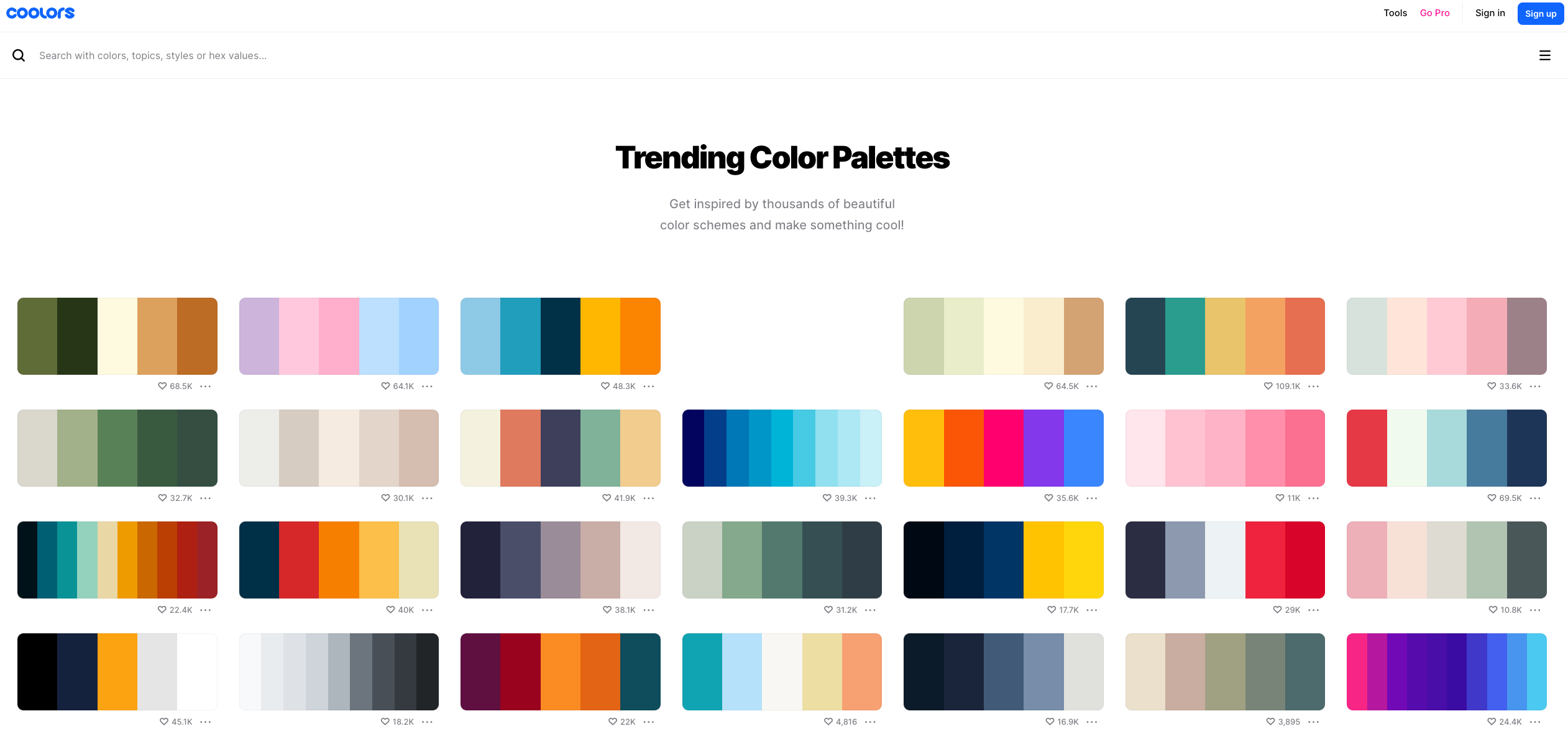
# Define colors in a list
colors = ['#9c575f', '#8763a3', '#c87081', '#51a09c', '#5186c4', '#32527a', '#e58879', '#c5a279', '#637b4c']

# Plot the stacked area plot
ax.stackplot(df.index, df.T, labels=df.columns, colors=colors, alpha=0.9)

---

4 The Professional Look

Adding a few more features to our graph will make it look way more professional. They will go on top of any graphs and are independent of the data we are using in this article. Thanks to the code snippet below, these adjustments will take little to no effort to implement. Author's advice: save it and re-use it at will. The reader can tweak them to create their own visual identity.

• Spines The spines make up the box visible around the graph. They are removed, except for the left one which is set to be a bit thicker.

• Red line and rectangle on top A red line and rectangle are added above the title to nicely isolate the graph from the text above it.

• Title and subtitle What is a graph without a title to introduce it? The subtitle can be used to further explain the content or even present a first conclusion.

• SourceA must have, in all charts ever produced.

• Margin adjustments The margins surrounding the graph area are adjusted to make sure all the space available is used.

• White background Setting a white background (from transparent by default) will be useful when sending the chart via emails, Teams or any other tool, where a transparent background can be problematic.

# Remove the spines
ax.spines[['top','right','bottom']].set_visible(False)

# Make the left spine thicker
ax.spines['left'].set_linewidth(1.1)

# Add in red line and rectangle on top
ax.plot([0.05, .90], [.98, .98], transform=fig.transFigure, clip_on=False, color='#E3120B', linewidth=.6)
ax.add_patch(plt.Rectangle((0.05,.98), 0.04, -0.02, facecolor='#E3120B', transform=fig.transFigure, clip_on=False, linewidth = 0))

# Add in title and subtitle
ax.text(x=0.05, y=.93, s="Electricity Production by Source in the United States", transform=fig.transFigure, ha='left', fontsize=14, weight='bold', alpha=.8)
ax.text(x=0.05, y=.90, s="Evolution of the electricity production by source in the US from 1985 to 2022", transform=fig.transFigure, ha='left', fontsize=12, alpha=.8)

# Set source text
ax.text(x=0.1, y=0.12, s="Source: Ember - Yearly Electricity Data (2023); Ember - European Electricity Review (2022); Energy Institute - Statistical Review of World Energy (2023)", transform=fig.transFigure, ha='left', fontsize=10, alpha=.7)

# Adjust the margins around the plot area
plt.subplots_adjust(left=None, bottom=0.2, right=None, top=0.85, wspace=None, hspace=None)

# Set a white background
fig.patch.set_facecolor('white')

---

5 The Final Touch

To get to the end result, introduced at the beginning of the article, the only thing left to do to is to reshape the legend which is very much in the way for now.

Placing this code snippet right after the y-axis reformatting will do the trick.

# Position the legend above the graph and spread horizontally
legend = ax.legend(loc='upper center', bbox_to_anchor=(0.5, +1.10), ncol=len(df.columns), frameon=False, columnspacing=0.75)
legend.get_lines()[::-1]

---

6 Final Thoughts

The intent of this article was to share the knowledge gathered here and there to build a more compelling stacked area chart using Matplotlib. I tried to make it as practical as possible with re-usable code snippets.

I am sure there are other adjustments to be made that I did not think of. If you have any improvement ideas, feel free to comment and make this article more useful to all!

This article only focused on stacked area charts, stay tuned for more!

Thanks for reading all the way to the end of the article. Follow for more! Feel free to leave a message below, or reach out to me through LinkedIn / X if you have any questions / remarks!

Get an email whenever Guillaume Weingertner publishes.

Tags: Area Chart Data Science Data Visualization Matplotlib Python

Comment