A Deep Dive into Odds Ratio
PART 1 OF THE DEEP DIVE INTO ODDS RATIOS SERIES

You have probably heard a sentence similar to this: "Smokers are five times more likely to develop lung cancer." Although this example is not from a real study and is intended for illustrative purposes only, it serves as a good starting point for our discussion about odds ratios.
Not a Medium member yet? Continue using this free version!
The odds ratio is a relatively simple concept and, in practice, is also easy to interpret. In this article, we will discuss odds and odds ratios, provide a clear step-by-step explanation of the calculations, and demonstrate a quick method using the SciPy library in Python. Finally, we will explore how to communicate and interpret odds ratios effectively.
What is Odds Ratio?
I use the example above because odds ratios have a significant application in clinical research to quantify the relationship between exposure and outcome. As the name suggests, the odds ratio compares the odds of an event (or disease) occurring in the exposed group to the odds of the event occurring in the unexposed group [1].
But what are odds, anyway? In essence, the odds are a ratio of the probability of an outcome occurring to the probability of it not occurring [2]. For example, if the probability of mortality is 0.3, then the odds are calculated as follows: odds = p / (1-p) = 0.3 / (1 – 0.3) = 0.43
It's important to recognize that odds and probability have different meanings; however, when the probability is very small, they yield similar results. For example, if we change the probability to 0.05, the odds are calculated as: odds = p / (1-p) = 0.05 / (1–0.05) = 0.052. This occurs because the probability of the outcome not occurring is nearly 1 (remember, probabilities range from 0 to 1).
Odds and odds ratio in product analytics
I assume that most of my readers come from the product or business analytics field, so you might be asking how we can apply the methodologies discussed above to our domain.
If you search for "odds ratio" on Google, you will likely find numerous scientific articles from medical or clinical studies. Despite this, we can borrow the concept as a tool to enhance our decision-making approach.
Let's say you are a data analyst or a product manager for a company focused on SaaS products. One of the products offers both free and paid subscriptions. Since one of the success metrics is the number of users who convert to paid membership within 7 days after signing up, you should be interested in identifying the factors that potentially drive users to convert during this time window.
We can hypothesize that trial usage of one of the premium features may lead users to convert. The odds ratio can be used to validate this hypothesis by examining the relationship between the usage of the premium feature by newly signed-up users and the likelihood of those users converting to paid membership within 7 days.
Returning to the definition of odds ratio, we can adapt it to our case as follows:
- Odds Ratio: The odds ratio compares the odds of users converting within 7 days who used the premium feature trial to the odds of users converting within 7 days who did not use the premium feature at all.
- Odds: The odds represent the probability of users who used the premium feature trial converting to paid membership compared to those who did not convert. A similar definition applies to users who did not use the premium feature trial.
What does the value means?
We should expect the conclusion to be something like, "Users who use the premium feature are XX times more likely to convert to paid membership."
The goal is to determine the XX value, which represents the odds ratio itself. However, it is important to understand the implications of this value.
When the odds ratio is equal to 1, it indicates that there is no difference between users who adopted the premium feature and those who did not. In other words, there is no association between using the premium feature and converting to paid membership within 7 days.
Conversely, when the odds ratio is above or below 1, it indicates that adoption of the premium feature is associated with higher or lower odds of the outcome, respectively.
Calculate Odds Ratio… the hard way
Import libraries
First things first, we need to import the holy trinity of Python packages: Pandas, NumPy, and Matplotlib. We will use these three fundamental libraries as we start by calculating the odds ratio from scratch, or, in my version, in a hard way.
import pandas as pd
import numpy as np
import matplotlib.pyplot as plt
Prepare the dataset
From the example we used earlier, let's examine how to calculate the odds ratio. We will utilize a Python-generated dataset, with the details and the code provided at the end of the article. The dataset consists of three columns (and we will later include additional columns): user_id, usage_of_premium_feature and converted_to_paid_in_7_days.
data = generate_dataset(n=1000)
print(data[['user_id', 'usage_of_premium_feature', 'converted_to_paid_in_7_days']])
user_id usage_of_premium_feature converted_to_paid_in_7_days
0 1 False False
1 2 True True
2 3 True True
3 4 True True
4 5 False False
.. ... ... ...
995 996 False False
996 997 True False
997 998 False False
998 999 True True
999 1000 False True
[1000 rows x 3 columns]user_id: A unique identifier assigned to each user in the dataset.usage_of_premium_feature: A boolean variable indicating whether a user has used the trial of the premium feature during the 7 days after signing up. If the user uses the premium feature after converting to a paid member, it will not be counted as True.converted_to_paid_in_7_days: A boolean variable indicating whether a user converted to a paid subscriber within 7 days after first signing up. If the user converted to a paid subscriber beyond this period, it will not be counted as True.
Pretty simple dataset, right? This is the minimum information we need to conduct the odds ratio calculation.
Create a contingency table
From the dataset, we can identify four types of users, as listed below. I have simplified the naming for clarity, and I'm confident that we can understand the complete context of each condition:
- Converted with premium feature
- Converted without premium feature
- Not converted with premium feature
- Not converted without premium feature
Now, let's count each type from the dataset.
converted_with_premium = data[(data['usage_of_premium_feature']) & (data['converted_to_paid_in_7_days'])]['user_id'].nunique()
converted_without_premium = data[(~data['usage_of_premium_feature']) & (data['converted_to_paid_in_7_days'])]['user_id'].nunique()

not_converted_with_premium = data[(data['usage_of_premium_feature']) & (~data['converted_to_paid_in_7_days'])]['user_id'].nunique()
not_converted_without_premium = data[~(data['usage_of_premium_feature']) & (~data['converted_to_paid_in_7_days'])]['user_id'].nunique()

# Print the counts
print(f"Converted with Premium Feature: {converted_with_premium}")
print(f"Not Converted with Premium Feature: {not_converted_with_premium}")
print(f"Converted without Premium Feature: {converted_without_premium}")
print(f"Not Converted without Premium Feature: {not_converted_without_premium}")
Converted with Premium Feature: 402
Not Converted with Premium Feature: 95
Converted without Premium Feature: 210
Not Converted without Premium Feature: 293In odds ratio analysis, the numbers described above are typically organized into a contingency table. A contingency table simply shows the frequency of each combination in a two-by-two format (the simplest version).

The two-by-two table provides values for a, b, c, and d, which correspond to the conditions we outlined earlier.
a --> Converted with Premium Feature: 402
b --> Not Converted with Premium Feature: 95
c --> Converted without Premium Feature: 210
d --> Not Converted without Premium Feature: 293
In Python, we can utilize the crosstab() function from the pandas library to create a contingency table. Additionally, we can use the Categorical() function to ensure that the order of the categories is correct (i.e., [True, False]).
contingency_table = pd.crosstab(
    pd.Categorical(data['usage_of_premium_feature'], categories=[True, False], ordered=True),
    pd.Categorical(data['converted_to_paid_in_7_days'], categories=[True, False], ordered=True),
    colnames=['Converted in 7D'],
    rownames=['Premium Feature']
)

print(contingency_table)
Converted in 7D True False
Premium Feature
True 402 95
False 210 293Note: The reason I am presenting two methods here is to reduce our dependency on a single programming language, in case we need to build the contingency table in an environment where there is no straightforward way to achieve this. Similarly, in the following sections, we will demonstrate methods that can be implemented on any platform.
Calculate odds of each segment
The counts of each condition in the contingency table will be used to calculate the odds for each segment: the odds of users with the premium feature and the odds of users without the premium feature.
Both odds are calculated by dividing the number of users who converted by the number of users who did not convert. Referring back to the contingency table, the calculations would be as follows:
Odds of users with the premium feature = a / c
Odds of users without the premium feature = b / d
Let's implement this in Python by creating a function called calculate_odds()
def calculate_odds(count_of_event, count_of_non_event):
    return count_of_event / count_of_non_event

odds_with_premium = calculate_odds(converted_with_premium, not_converted_with_premium)
odds_without_premium = calculate_odds(converted_without_premium, not_converted_without_premium)

print(f"Odds of User with Premium Feature: {odds_with_premium}")
print(f"Odds of User without Premium Feature: {odds_without_premium}")
Odds of User with Premium Feature: 4.231578947368421
Odds of User without Premium Feature: 0.7167235494880546From the calculations above, we can see that the odds of a user who uses the premium feature are 4.231, while the odds of a user who does not use the premium feature are 0.716.
Calculate odds ratio
Finally, after calculating the odds for each segment, we can easily compare the odds of the segment with exposure (in this case, using the premium feature) to the odds of the segment without exposure.
If you prefer to refer back to the contingency table, here's how to derive the final formula for the odds ratio:
Odds ratio = (Odds of users with premium feature) / (Odds of users without premium feature) Odds ratio = (a / c) / (b / d) Odds ratio = (a d ) / ( b c)
In the Python code, we will define this calculation in a function called calculate_odds_ratio() as follows:
def calculate_odds_ratio (odds_of_exposure, odds_of_non_exposure):
    return odds_of_exposure / odds_of_non_exposure

odds_ratio_premium_feature = calculate_odds_ratio(odds_with_premium, odds_without_premium)

print(f"Odds Ratio (Premium Feature Usage vs Non-Usage): {odds_ratio_premium_feature}")
Odds Ratio (Premium Feature Usage vs Non-Usage): 5.90406015037594The result shows that the odds ratio is 5.90, which means that users who used the premium feature are 5.90 times more likely to convert to paid membership within 7 days after signing up compared to users who did not use the premium feature.
As someone who deals with data daily, you might be wondering: is this statistically significant? We can use confidence intervals to assess the significance of the odds ratio.
95% Confidence Interval of Odds Ratio
The confidence interval for the odds ratio can be calculated by first determining the confidence interval for log(OR) [3]. The formula is as follows:
CI of log(OR) = log(OR) ± Z × SE(log(OR))
Where Z is the critical value for the desired confidence interval. For a 95% confidence interval, we use Z = 1.96.
After completing the calculation, we can exponentiate the result to obtain the confidence interval for the odds ratio:
Upper CI of OR = e^(log(OR) + Z × SE(log(OR)))
Lower CI of OR = e^(log(OR) – Z × SE(log(OR)))
The standard error of log(OR) (SE(log(OR))) can be estimated using the following formula based on the four frequencies in the contingency table:
SE(log(OR)) = √(1/a + 1/b + 1/c + 1/d)
Now, let's calculate this in Python.
def calculate_std_err_log_or(a, b, c, d):
    return np.sqrt(1/a + 1/b + 1/c + 1/d)

def calculate_confint_odds_ratio(odds_ratio, a, b, c, d):
    z = 1.96

    std_err_log_or = calculate_std_err_log_or(a, b, c, d)
    confint_lower_log_or = np.log(odds_ratio) - z * std_err_log_or
    confint_uppper_log_or = np.log(odds_ratio) + z * std_err_log_or

    confint_lower_or = np.exp(confint_lower_log_or)
    confint_upper_or = np.exp(confint_uppper_log_or)

    return confint_lower_or, confint_upper_or

a = contingency_table.loc[True, True]
b = contingency_table.loc[False, True]
c = contingency_table.loc[True, False]
d = contingency_table.loc[False, False]

lower_confint, upper_confint = calculate_confint_odds_ratio(odds_ratio_premium_feature, a, b, c, d)
print(f"Odds Ratio   : {odds_ratio_premium_feature}")
print(f"Lower 95% CI : {lower_confint}")
print(f"Upper 95% CI : {upper_confint}")
Odds Ratio : 5.90406015037594
Lower 95% CI : 4.438585231409555
Upper 95% CI : 7.8533867081307305Well, we have determined that the 95% confidence interval for the odds ratio is from 4.43 to 7.85. But what does this mean?
Previously, we noted that if the odds ratio is equal to one, it indicates that there is no difference between users who adopted the premium feature and those who did not. Therefore, if the value of 1 falls between the lower and upper bounds of the confidence interval for the odds ratio, we can conclude that the result is not statistically significant, meaning no difference has been observed.
In our case, since the confidence interval ranges from 4.43 to 7.85, which does not include the value of 1, we can confidently say that the result is statistically significant.
Calculate Odds Ratio using Python Library
It's been a long journey, but hopefully, it will be worthwhile. I want to remind you again that understanding this process the hard way makes us less dependent on any specific platform. However, if you're using Python for your analysis, there's a library that allows us to perform this calculation in just one or two lines.
First, make sure you have installed SciPy by using the following command:
pip install scipyThen, import the necessary function as follows:
from scipy.stats.contingency import odds_ratioThe next step is essentially the same as before until we obtain the contingency table, which will then serve as the input to the odds_ratio() function. It is always important to ensure that the contingency table follows the format we've discussed earlier. Therefore, regardless of the method you use, defining the contingency table with the correct order of the columns and rows is crucial.
data = generate_dataset(n=1000)

contingency_table = pd.crosstab(
    pd.Categorical(data['usage_of_premium_feature'], categories=[True, False], ordered=True),
    pd.Categorical(data['converted_to_paid_in_7_days'], categories=[True, False], ordered=True),
    colnames=['Converted in 7D'],
    rownames=['Premium Feature']
)

res = odds_ratio(contingency_table, kind='sample')
odds_ratio_res = res.statistic
lower_confint, upper_confint = res.confidence_interval(confidence_level=0.95)

print(f"Odds Ratio   : {odds_ratio_res}")
print(f"Lower 95% CI : {lower_confint}")
print(f"Upper 95% CI : {upper_confint}")
and here is the result
Odds Ratio   : 5.90406015037594
Lower 95% CI : 4.438608500925912
Upper 95% CI : 7.853345536554002
The result is pretty much the same with the result for our manual calculation.
In SciPy's documentation for this function, two methods are provided for calculating the odds ratio.. First is 'sample' method, which we just use here and secondly is the default 'conditional' method.
Essentially, the first method calculates the odds ratio in the same manner as demonstrated earlier, using the counts from the contingency table. In contrast, the second method employs a more advanced statistical technique, making it more accurate for smaller sample sizes. For further explanation, you can refer to the documentation provided.
So, let's explore what happens if we use the 'conditional'method instead.
res = odds_ratio(contingency_table, kind='conditional')
odds_ratio_res = res.statistic
lower_confint, upper_confint = res.confidence_interval(confidence_level=0.95)

print(f"Odds Ratio   : {odds_ratio_res}")
print(f"Lower 95% CI : {lower_confint}")
print(f"Upper 95% CI : {upper_confint}")
Odds Ratio : 5.892471038481242
Lower 95% CI : 4.397617702070802
Upper 95% CI : 7.9425384158360695We can observe a very small difference between 'conditional' to 'sample' method: 5.892 vs 5.904, which is only about 0.19%. However, since the 'conditional' method is more robust, especially when dealing with small samples, it is recommended to use it when utilizing the SciPy package. Alternatively, when we need to calculate from scratch, we can simply use the straightforward method demonstrated earlier
Visualize the Odds Ratio
Odds ratio in text
The most common way to present the odds ratio is by stating the odds ratio value along with the 95% confidence interval to assess whether the result is statistically significant.
In the example below, I directly quote the abstract from the article by Yang Y, et al. [4], which presents the odds ratio and its confidence interval in a sentence. We will not delve deeply into the research; instead, we will focus on how the odds ratio is presented.
A total of 127 patients exhibited poor functional outcomes. Following comprehensive adjustments, those in the highest SHR tertile had a significantly increased risk of poor prognosis compared to those in the lowest tertile (odds ratio [OR], 4.12; 95% confidence interval [CI]: 1.87–9.06). Moreover, each unit increase in SHR was associated with a 7.51-fold increase in the risk of poor prognosis (OR, 7.51; 95% CI: 3.19–17.70).
We can see that the odds ratio and confidence interval have been mentioned twice. This is quite straightforward, especially for readers who are already familiar with the concept of odds ratios.
While the information can also be presented using a table or chart, I believe it is not strictly necessary; having a clear number for the odds ratio is more important for understanding its significance in a single value.
Odds ratio in visualization
On the other hand, if we want to show a comparison of odds ratios for categorical variables, I recommend checking out this excellent blog post by Henry Lau [5], titled "Against all odds – how to visualise odds ratios to non-expert audiences". In this post, he discusses how the Office of National Statistics (ONS) communicates the odds ratios of different ethnic groups compared to the white ethnicity.
Let's return to our previous case. To maximize our product's reach to a larger user base, we leverage multiple marketing channels. Initially, most users came through organic search, and then we scaled our user base through paid ads, referrals, and email campaigns.
Inspired by the blog, we want to compare the new channels against organic search as a baseline. To achieve this, we can calculate the odds ratio by comparing each channel (paid ads, referrals, and email campaigns) to organic search.
data = generate_dataset(n=1000)
channels_to_compare = ['Paid Ads', 'Referral', 'Email Campaign']
results = []

for channel in channels_to_compare:
    data_sliced = data[data['marketing_source'].isin(['Organic', channel])][['marketing_source', 'converted_to_paid_in_7_days']]
    contingency_table = pd.crosstab(
        pd.Categorical(data['marketing_source'], categories=[channel, 'Organic'], ordered=True),
        pd.Categorical(data['converted_to_paid_in_7_days'], categories=[True, False], ordered=True),
        colnames=['Converted in 7D'],
        rownames=['Marketing Source']
    )

    res = odds_ratio(contingency_table)
    odds_ratio_res = res.statistic
    lower_confint, upper_confint = res.confidence_interval(confidence_level=0.95)

    results.append({
        'channel' : channel,
        'odds_ratio' : odds_ratio_res,
        'lower_confint' : lower_confint,
        'upper_confint' : upper_confint
    })

df_result = pd.DataFrame(results)
print(df_result)
channel odds_ratio lower_confint upper_confint
0 Paid Ads 0.482623 0.339595 0.683895
1 Referral 2.240552 1.473594 3.444094
2 Email Campaign 0.707163 0.482963 1.034957After obtaining the odds ratio and confidence interval for each channel, the next step is to plot the results, which will generally follow the approach outlined in the blog mentioned above.
def plot_multiple_odds_ratio(data, cat_col, or_col, lower_confint_col, upper_confint_col, comparison_group='Organic search'):
    import matplotlib.pyplot as plt

    color_dict = {
        'blue': '#1f77b4',
        'red': '#d62728',
        'green': '#2ca02c',
        'brown': '#8c564b',
        'cyan': '#17becf',
        'gray': '#7f7f7f'
    }

    x = data[or_col]
    y = data[cat_col]
    confint = [data[lower_confint_col], data[upper_confint_col]]

    plt.figure(figsize=(8,4))

    # Plot the Odds Ratios as dots with Confidence Intervals
    plt.errorbar(
        x=x, y=y, xerr=[x-confint[0], confint[1]-x],
        fmt='o', color=color_dict['blue'], ecolor=color_dict['blue'], capsize=5, linestyle='None'
    )

    # Add a reference line for OR = 1
    plt.axvline(x=1, color=color_dict['gray'], linestyle='-')

    # Custom x-tick values and more descriptive labels
    xticks = [0, 0.5] + [i for i in range(1, int(np.ceil(max(x)))+1)]
    xtick_labels = ['', '0.5x', 'Just as likely'] + [f'{i}x as likely' for i in range(2, int(np.ceil(max(x)))+1)]
    plt.xticks(xticks, xtick_labels)
    plt.xlabel(f'')

    plt.grid(visible=True, axis='x')
    plt.gca().spines['top'].set_visible(False)
    plt.gca().spines['right'].set_visible(False)
    plt.tick_params(axis='both', which='both', pad=10,length=0)

    plt.suptitle(f'Likelihood compared to {comparison_group}', fontweight='bold')
    plt.tick_params(axis='both', which='both', length=0)
    plt.tight_layout()
    plt.show()

plot_multiple_odds_ratio(
    data=df_result,
    cat_col='channel',
    or_col='odds_ratio',
    lower_confint_col='lower_confint',
    upper_confint_col='upper_confint',
    comparison_group='Organic search'
)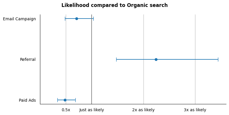
As the result, we have a simple yet informative chart that illustrates the comparison of odds ratios, or the likelihood of converting to a paid subscription, between different channels compared to organic search.
The chart clearly shows that referrals are more than twice as likely to convert compared to organic search. This insight prompts us to explore how to further invest in this channel for effective marketing.
Next, we have the email campaign channel. As discussed earlier, the benefit of the confidence interval is to assess the significance of the odds ratio. In this case, the odds ratio for email campaigns appears to be less than 1, which is not favorable. However, the confidence interval spans include OR = 1, indicating that this result is not statistically significant. Therefore, we cannot confidently conclude that email campaigns are less likely to convert compared to organic search.
Lastly, we have paid ads, which show a likelihood of 0.5x, meaning they are less likely to convert compared to organic search. The confidence interval indicates that this is different from the email campaign, as the odds ratio for paid ads being lower than 1 is statistically significant. This suggests that we should further investigate how to optimize the marketing budget for paid ads, such as evaluating ad targeting.
Conclusion
Throughout this article, we explored the concept of odds ratios in detail. We started with the concept of odds itself, discussed step-by-step calculations, and demonstrated how to use the SciPy library for a more robust and effective approach. We also covered how to visualize and interpret the results of the odds ratio.
This article used an imaginary use case of internal data analysis to examine the factors that contribute to user conversion to paid membership. However, the application of odds ratios is not limited to internal data analysis alone.
Odds ratios are often used to encourage users to take actions that increase their likelihood of receiving a benefit. For example, on a job platform site, you might find an ad that said "If you are a premium user, your chances of getting a job are three times higher than those of a free user". While I cannot confirm that the method they used is an odds ratio, it is quite likely that this is the case.
In the next article, I will bridge the gap from odds ratios to logistic regression. Initially, I planned to cover everything in one article; however, discussing odds ratios alone has already turned into quite a lengthy topic.
Part 2 of this series is ready to read:
So if you found this article helpful and interesting, please follow me on Medium for more content on similar topics.
