Addressing the Butterfly Effect: Data Assimilation Using Ensemble Kalman Filter

1. Quick Start: Why Data Assimilation
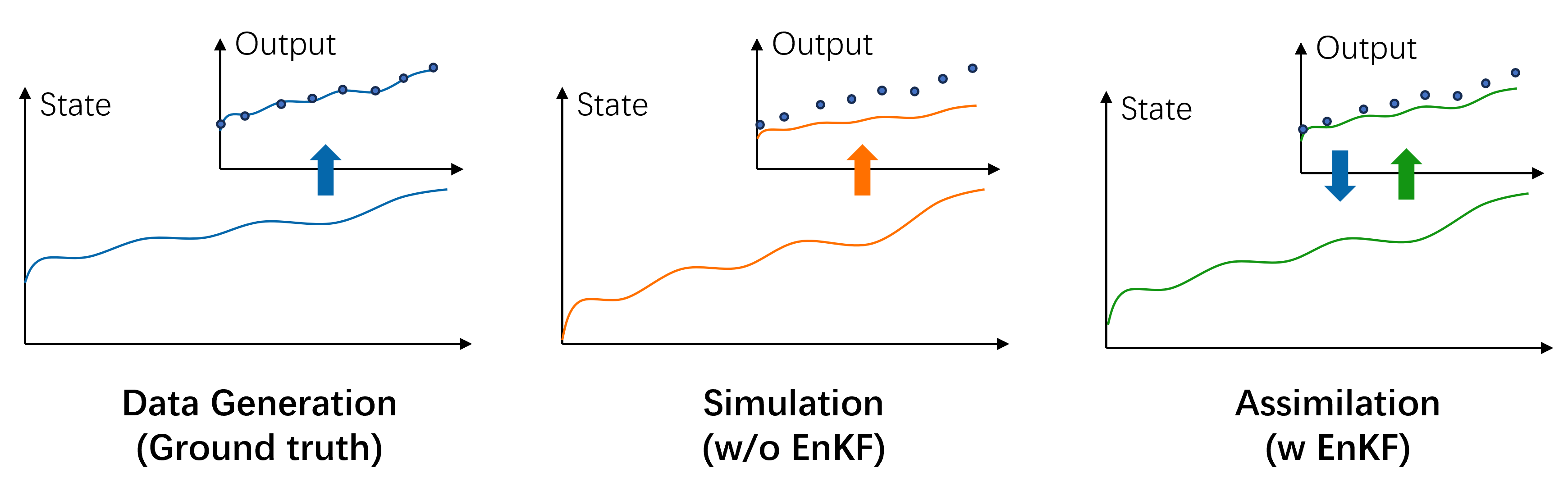
Many real-world dynamical systems are chaotic, where small changes in initial conditions lead to significant differences in later states. This phenomenon, also known as the Butterfly Effect, makes it challenging for programmed physical models to predict system behaviors accurately. Data assimilation addresses this issue by integrating observations into model state estimation. It is commonly applied to time-series prediction problems, especially in physical system models like weather forecasting. The Ensemble Kalman Filter (EnKF) is a widely used algorithm in data assimilation with elegant theory and simple implementation, which gains popularity from science to industry.

This post serves as a tutorial on EnKF. It will introduces the basic mathematics of EnKF, provide step-by-step code, and showcase the practical implementation using a toy case. The tutorial is structured as follows:
- 1. Quick Start: Why Data Assimilation
- 2. Prerequisites
- 3. Problem Overview
- 4. How EnKF Works
- 5. EnKF Implementation
- 6. Case Study
- 7. Summary
- 8. Further Reading
2. Prerequisites
A basic understanding of college-level statistics and linear algebra is sufficient. Feel free to skip the math section if you're only interested in testing the algorithm. Experience with Python and NumPy is required. The code repository can be found in https://github.com/YANGOnion/python-data-assimilation-tutorial.
3. Problem Overview
This tutorial uses rainfall-runoff modeling as a case study, which is a typical time-series prediction problem. The model is simplified to a bucket, where storage first receives rainfall input and experiences evaporation loss, then releases runoff based on the storage level. Rainfall and evaporation rates are the system's "external inputs", water storage is the system state, and runoff is the observable output.

Due to the model's limited ability to capture the complex real-world processes, discrepancies exist between the simulated and true states, which are later transferred to the output residuals. Data assimilation helps improve the simulation of the output variable by adjusting state values based on real-time output observations. In this tutorial, we manually generate "ground truth" data for the system and compare it with both the simulated and assimilated data, aiming to demonstrate the improvements achieved with EnKF.
4. How EnKF Works
4.1. Bayesian Interpretation of Kalman Filter
Data assimilation determines how much model states should be updated based on the observed model output. Sounds familiar? It actually aligns with the idea of Bayesian inference. According to the Bayes' rule:

where x is the model states and y is the model output. The simulation model consists of two functions, a state transition model m and an observation operator h:

Using Gaussian prior distribution p(x) and likelihood p(y|x), we have:

The posterior distribution can be derived as:

Here the Kalman Gain K balances how much we trust in the model verse the observations. The procedure above for updating model states x is called the Kalman Filter (KF).
4.2. Ensemble Kalman Filter
KF has two major limitations: (1) If model states have extremely high dimensions, we have to store a large covariance matrix of x and conduct intense matrix multiplications. (2) If the observation operator h is nonlinear, the variance of y and the covariance between x and y can not be explicitly calculated. EnKF solves these two problems by using Monte Carlo sampling of model states. The EnKF procedure is as follows:
- Initialization: Create a ensemble of model states and collect observations:

- Forecast step: Propagate each ensemble member through the state transition to get the prior model states, and then compute the corresponding output:

- Observation update: Calculate the Kalman Gain K:

- Analysis step: Update the ensemble members, resulting in the posterior model states:

- Iteration: Initialize the ensemble for next EnKF time step:

Since covariance matrices are calculated empirically from a small ensemble of data, EnKF avoids extensive data storage and algebra computation. Additionally, EnKF relaxes the requirement for a linear observation operator in the KF method.
5. EnKF Implementation
First import necessary libraries:
import numpy as np
from numpy.typing import NDArray
from typing import Tuple
import matplotlib.pyplot as pltpy
5.1. EnKF Update Step
In an EnKF update step, the posterior ensemble of states from the previous step and the observations from the current step are used to update the current ensemble of states. We define a function to handle this update procedure:
def enkf_update(ensemble: NDArray[Tuple[float, float]],
                observation: NDArray[float],
                model: callable,
                obs_operator: callable,
                R: NDArray[Tuple[float, float]],
                **kwargs
                ) -> NDArray[Tuple[float, float]]:
    '''
    :param ensemble: (ensemble_size, state_dim)
    :param observation: (y_dim, )
    :param model: state transition
    :param obs_operator: observation operator
    :param R: (y_dim, y_dim)
    :param kwargs: external input for the state transition model
    :return: updated ensemble
    '''
    # Forecast step
    forecast_ensemble = np.array([model(state, **kwargs) for state in ensemble])
    H_ensemble = np.array([obs_operator(state) for state in forecast_ensemble])

    # Compute the empirical covariance
    P_f_xy = (forecast_ensemble - forecast_ensemble.mean(axis=0)).T @ (H_ensemble - H_ensemble.mean(axis=0)) / (forecast_ensemble.shape[0] - 1)
    P_f_yy = np.cov(H_ensemble.T)

    # Kalman gain
    K = P_f_xy @ np.linalg.inv(P_f_yy + R)

    # Analysis step
    update_ensemble = np.empty_like(ensemble)
    for i in range(ensemble.shape[0]):
        innovation = observation - H_ensemble[i]
        update_ensemble[i] = forecast_ensemble[i] + K @ innovation

    return update_ensemble
5.2. EnKF Loop
In a time-series prediction problem, such as rainfall-runoff modeling, EnKF runs continuously for each time step, using the updated ensemble of states from the last step. The following function executes EnKF over a period and returns the updated state ensembles for all time steps.
def enkf_loop(initial_ensemble: NDArray[Tuple[float, float]],
              observations_y: NDArray[Tuple[float, float]],
              R: NDArray[Tuple[float, float]],
              model: callable,
              obs_operator: callable,
              model_input: dict[str, NDArray[Tuple[float, float]]],
              inflation_noise_std: float
              ) -> NDArray[Tuple[float, float, float]]:
    '''
    :param initial_ensemble: (ensemble_size, state_dim)
    :param observations_y: (time_steps, y_dim)
    :param R: (y_dim, y_dim)
    :param model: state transition
    :param obs_operator: observation operator
    :param model_input: dict of (time_steps, input_dim), external input for the state transition model
    :param inflation_noise_std: standard deviation of inflation noise
    :return: updated ensemble results (time_steps, ensemble_size, state_dim)
    '''
    ensemble = initial_ensemble.copy()
    ensemble_history = []
    for t in range(time_steps):
        observation = observations_y[t]
        step_model_input = {k: v[t] for k, v in model_input.items()}
        ensemble = enkf_update(
            ensemble=ensemble,
            observation=observation,
            model=model,
            obs_operator=obs_operator,
            R=R,
            **step_model_input
        )
        # Add inflation noise to avoid ensemble collapse
        ensemble += np.random.normal(0, inflation_noise_std, size=ensemble.shape)
        ensemble_history.append(ensemble.copy())
    ensemble_history = np.array(ensemble_history)
    return ensemble_history
Note that we add certain randomness, i.e., "inflation noise", to the updated ensemble, which prevents the ensemble from collapsing into a narrow range due to the propagation of covariance underestimation over time.
6. Case Study
6.1. Data Generation
First, we define functions to generate synthetic "ground truth" for the states and output observations in the rainfall-runoff modeling case. The function true_state_transition is the true system process of model m, and true_observation_operator is the true system process of model h that generates observations with measurement noises. These functions are unseen during the assimilation process.
def true_state_transition(states: NDArray[float], rainfall: NDArray[float], evap_coeff: NDArray[float]) -> NDArray[
    float]:
    '''
    :param states: (state_dim, )
    :param rainfall: (state_dim, )
    :param evap_coeff: (state_dim, )
    :return: (state_dim, )
    '''
    updated_states = states + rainfall - evap_coeff * states
    updated_states = np.maximum(updated_states, 0)  # Ensure non-negative states
    updated_states = np.minimum(updated_states, 50)  # Maximum state
    return updated_states

def true_observation_operator(states: NDArray[float], measure_noise_std: float) -> NDArray[float]:
    '''
    :param states: (state_dim, )
    :return: (y_dim, )
    '''
    # Non-linear relationship
    y = np.array([(states.clip(0) ** 0.5).sum()])
    y += np.random.normal(0, measure_noise_std, size=len(y))
    return *
We also have simulation models for m (state_transition) and h (observation_operator) in the rainfall-runoff modeling case. These models are approximates the system process and are subject to representative errors. This means, they simulate the states and output variable with certain discrepancy to the true values generated by true_state_transition and true_observation_operator.
def state_transition(states: NDArray[float], rainfall: NDArray[float], evap_coeff: NDArray[float]) -> NDArray[float]:
    updated_states = states ** 0.99 * 1.01 + rainfall * 1.02 - evap_coeff * states
    updated_states = np.maximum(updated_states, 0)  # Ensure non-negative states
    updated_states = np.minimum(updated_states, 50)  # Maximum state
    return updated_states

def observation_operator(states: NDArray[float]) -> NDArray[float]:
    y = np.array([(states.clip(0) ** 0.5).sum()])
    return y
Using these functions and synthetic external inputs – rainfall data (rainfall_data) and evaporation rate (evap_coef_data)—the following code produces the ground truth model states (true_states) and output observations (observations_y), as well as the simulated model states (sim_states) and output (simulations_y).
def generate_data(time_steps: int, state_dim: int, measure_noise_std: float):
    rainfall_data = np.random.uniform(0, 20, size=(time_steps, state_dim))
    rainfall_data = (rainfall_data - 10).clip(min=0)
    evap_coef_data = np.random.uniform(0.05, 0.1, size=state_dim)
    evap_coef_data = np.repeat(evap_coef_data[:, None], time_steps, axis=1).T

    # Initialize variables
    true_state_list = [np.random.uniform(20, 40, size=state_dim)]  # Initial true state
    sim_state_list = [np.random.uniform(20, 40, size=state_dim)]  # Initial simulated state

    # Simulate true states and observations
    obs_y_list = []
    sim_y_list = []
    for t in range(time_steps):
        # Synthetic true states and simulated states
        true_state = true_state_transition(true_state_list[-1], rainfall_data[t], evap_coef_data[t])
        true_state_list.append(true_state)
        sim_state = state_transition(sim_state_list[-1], rainfall_data[t], evap_coef_data[t])
        sim_state_list.append(sim_state)
        # Synthetic observations and output simulations
        obs_y = true_observation_operator(true_state, measure_noise_std)
        obs_y_list.append(obs_y)
        sim_y = observation_operator(sim_state)
        sim_y_list.append(sim_y)

    true_states = np.array(true_state_list)
    sim_states = np.array(sim_state_list)
    observations_y = np.array(obs_y_list)
    simulations_y = np.array(sim_y_list)

    return rainfall_data, evap_coef_data, true_states[1:], sim_states[1:], observations_y, simulations_y

# Generate data
state_dim = 3
y_dim = 1
time_steps = 50
measure_noise_std = .5  # synthetic measurement error
rainfall_data, evap_coef_data, true_states, sim_states, observations_y, simulations_y = generate_data(time_steps, state_dim, measure_noise_std)
6.2. EnKF Application
We choose an ensemble size of 30 and run the EnKF with the randomly initialized ensemble to get the updated ensemble of model states for all time steps:
ensemble_size = 30
inflation_noise_std = 1.0  # synthetic inflation noise

# Initialization and data preparation
R = np.diag(np.repeat(measure_noise_std ** 2, y_dim))
initial_ensemble = np.random.uniform(10, 50, size=(ensemble_size, state_dim))
model = state_transition
obs_operator = observation_operator
model_input = {
    "rainfall": rainfall_data,
    "evap_coeff": evap_coef_data
}

# Run EnKF
ensemble_history = enkf_loop(initial_ensemble, observations_y, R, model, obs_operator, model_input, inflation_noise_std)
6.3. Evaluation
Finally, we compare the ground truth with the simulated and assimilated values respectively, for both model states and output variable. The following two figures show that the ground truth values are closer to the assimilated values than to the purely simulated values, demonstrating the effectiveness of EnKF in improving runoff modeling. Without EnKF, small differences between the simulated and true states amplify over time, illustrating a clear "butterfly effect".
# Plot state results
posterior_mean_ensembles = ensemble_history.mean(axis=1)
ci_lower = np.percentile(ensemble_history, 2.5, axis=1)
ci_upper = np.percentile(ensemble_history, 97.5, axis=1)
colors = plt.cm.viridis(np.linspace(0, 1, state_dim))
plt.figure(figsize=(12, 6))
for i in range(state_dim):
    plt.plot(true_states[:, i], label=f"True State {i + 1}", color=colors[i])
    plt.plot(sim_states[:, i], label=f"Simulated State {i + 1}", linestyle="dotted", color=colors[i])
    plt.plot(posterior_mean_ensembles[:, i], label=f"Posterior Mean State {i + 1}", linestyle="dashed", color=colors[i])
    plt.fill_between(range(time_steps), ci_lower[:, i], ci_upper[:, i], alpha=0.2, label=f"95% CI {i + 1}", color=colors[i])
plt.xlabel("Time Steps")
plt.ylabel("State Values")
plt.title("Model States during EnKF")
plt.legend()
plt.show()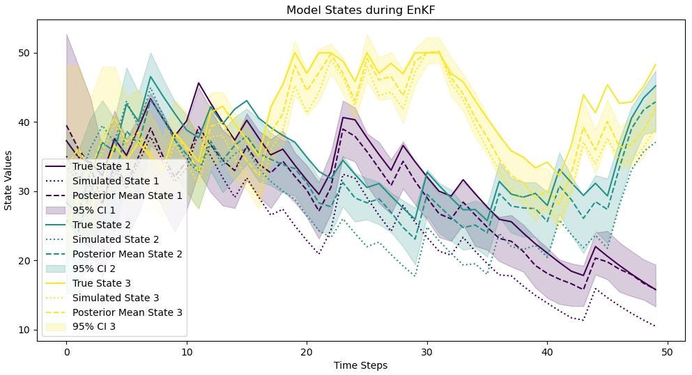
# Plot output y results
posterior_y = np.zeros((time_steps, ensemble_size, y_dim))
for t in range(time_steps):
    for i in range(ensemble_size):
        posterior_y[t, i] = observation_operator(ensemble_history[t][i])
posterior_mean_y = posterior_y.mean(axis=1)
ci_lower_y = np.percentile(posterior_y, 2.5, axis=1)
ci_upper_y = np.percentile(posterior_y, 97.5, axis=1)
colors = plt.cm.viridis(np.linspace(0, 1, y_dim))
plt.figure(figsize=(12, 6))
for i in range(y_dim):
    plt.plot(observations_y[:, i], label=f"Observation y {i + 1}", color=colors[i])
    plt.plot(simulations_y[:, i], label=f"Simulation y {i + 1}", linestyle="dotted", color=colors[i])
    plt.plot(posterior_mean_y[:, i], label=f"Posterior Mean y {i + 1}", linestyle="dashed", color=colors[i])
    plt.fill_between(range(time_steps), ci_lower_y[:, i], ci_upper_y[:, i], alpha=0.2, label=f"95% CI {i + 1}", color=colors[i])
plt.xlabel("Time Steps")
plt.ylabel("Observation Values")
plt.title("Output Variable during EnKF")
plt.legend()
plt.show()
7. Summary
Data assimilation helps address the "butterfly effect" in the physical simulation of dynamical systems. Through this post, you have learned the math behind the Ensemble Kalman Filter and applied it to solve a simple data assimilation problem with fewer than 200 lines of code. You are encouraged to replace the simulation model with those from your own study fields, even if they are highly complex physical models. You can also play with the code in more practical scenarios, such as multiple output variables and missing observations.
EnKF is not the only winner in data assimilation. Upcoming tutorials will explore other elegant algorithms, such as variational data assimilation. Please follow me on Medium to get updates on future articles.
