An Extensive Starters Guide For Causal Discovery using Bayesian Modeling

Author:Murphy | View: 24427 | Time: 2025-03-22 20:00:12

An Extensive Starter Guide For Causal Discovery Using Bayesian Modeling

. This extensive guide will walk you through applications, libraries, and dependencies of causal discovery approaches.

Landscape of Unsupervised Causal Discovery. Image by the author.

The endless possibilities of Bayesian techniques are also their weakness; the applications are enormous, and it can be troublesome to understand how techniques are related to different solutions and thus applications. In my previous blogs, I have written about various topics such as structure learning, parameter learning, inferences, and a comparative overview of different Bayesian libraries. In this blog post, I will walk you through the landscape of Bayesian applications, and describe how applications follow different causal discovery approaches. In other words, how do you create a causal network (Directed Acyclic Graph) using discrete or continuous datasets? Can you determine causal networks with(out) response/treatment variables? How do you decide which search methods to use such as PC, Hillclimbsearch, etc? After reading this blog you'll know where to start and how to select the most appropriate Bayesian techniques for causal discovery for your use case. Take your time, grab a coffee, and enjoy the read.

If you found this article about Bayesian Statistics useful, follow me to stay up-to-date with my latest content because I write more about this topic!

A Brief History

Bayesian methods are becoming "the new kid on the block" in the field of data science. To anticipate where the field of Bayesian is heading, it is good to know a bit of its history. It may not surprise you that Bayesian statistics have been around for a very long time. Let's start with Bayes himself – Thomas Bayes, to be precise. He formulated Bayes' theorem in a paper and published it in 1763 [1]. He laid the foundation for what we now know as Bayes' theorem. Then for a long time, Bayesian was in oblivion until the invention of Markov Chain Monte Carlo (MCMC) somewhere in the 50s to 60s. The invention of MCMC was thus crucial and brought approximations that allow estimating complex probability distributions when exact solutions are difficult or impossible to compute.

Time flies having fun because after 261 years we are still building new methods on top of the original work of Bayes.

What is Bayes' Theorem?

Bayes' Theorem forms the fundament for Bayesian networks. The Bayes rule itself is used to update model information, and can be stated as follows:

Equation: Bayes rule. Image by the author.

The equation contains four parts of probabilities. Let's go through each of them step by step. The most commonly used probability is the prior or belief probability. This probability is used by everyone and likely every day because it is the hypothesis before observing the evidence. In other words, it is our intuition or historical information that we have about a subject or system. As an example, A doctor might believe that a patient has a 20% chance of having a certain disease based on the patient's symptoms and age before any lab results come in. Or it is the chance that on a cloudy day, you believe with 80% chance it is going to rain and you bring an umbrella with you. Another probability in the equation is the conditional probability or likelihood. This is the probability of the evidence given that the hypothesis is true, which can be derived from the data. Then there is the marginal probability which describes the probability of new evidence under all possible hypotheses that need to be computed. Finally, the posterior probability is the probability that Z occurs given X. Read more about this in-depth over here:

A Step-by-Step Guide in detecting causal relationships using Bayesian Structure Learning in Python.

The Long Road to Popularity

Bayes or not Bayes, is this the question? Up to today, there is an ongoing debate between Bayesian and frequentist approaches. Which is the best? First of all, both approaches can determine patterns in the complete stack of information (data). One of the key differences is that only Bayesian statistics can include prior knowledge. This means that certain assumptions can be included upfront which will provide a head start and can make the analysis more reliable. This makes Bayesian analysis very powerful, especially in fields such as Medicine where there can be missing data about diseases, population, and treatment but where doctors have prior knowledge. In contradiction, the frequentist method requires choosing an experimental design in advance while Bayesian analysis is more flexible and you don't need to decide in advance.

For a long time, frequentist methods dominated because they have the property to make inferences on large sample sizes that are easier to compute than when using Bayesian methods. I experienced this myself in the early 2010s while working with genome-wide molecular data. I aimed to model thousands of features (gene expressions) to analyze the complex causal relationships related to treatment. To solve this, it required that the inferences involve complex integrals over high-dimensional probability distributions. Given the large datasets and limited computational power at the time, it was more practical to opt for statistical methods that offered closed-form solutions. This means that certain questions about causality on a genome-wide level could not be answered using Bayesian techniques at that time. At least not with limited computing power.

Bayesian techniques start to gain traction now! But we are not out of the woods yet.

The number of published medical articles using Bayesian statistics in the period from 1995 to 2018. Image by: https://www.ncbi.nlm.nih.gov/pmc/articles/PMC6406060/

Over the last few years, computing power has increased rapidly which may kickstart the use of Bayesian techniques to its full extent. But we are not out of the woods yet because, besides the computationally expensive methods, the next challenge is interpretability. Generally speaking, any technology, method, or statistic is meaningless if we don't know how to use, apply, or interpret it correctly.

While computing power is heavily increased, the new challenge for Bayesian techniques lies in effectively applying and interpreting the Bayesian statistics.

The Rise of Bayesian Thinking

Bayesian thinking is a natural way to update your understanding of a situation, making your conclusions more accurate as you gather more data. Many of the core fundamentals have been developed over centuries and mostly in academic settings. However, developments are nowadays also happening in the open-source community but also by the contribution of large companies. So besides the theoretical fundaments, we are increasingly seeing more frameworks that can be used to model Bayesian statistics.

We are heading towards the perfect storm for causal discovery. We have tons of data, scalable computing power, and powerful frameworks for Bayesian analysis.

In recent years, many industries have been working on implementing data-driven solutions for which machine-learning solutions were key. Nowadays we are stepwise more extending it towards data-driven decision-making. Data scientists recognize that incorporating prior knowledge into their models can improve predictions and lead to better results, especially in cases where interventions can be made for further optimizations. Examples of Bayesian techniques are those for improving statistical inference, developing Bayesian networks for complex decision-making, and Bayesian optimization techniques. In the next section, I will introduce some real-world applications that can be modeled using Bayesian techniques. If you need more background about Bayesian libraries and their differences, I recommend reading the following blog:

The Power of Bayesian Causal Inference: A Comparative Analysis of Libraries to Reveal Hidden…

The Landscape for Causal Discovery

The landscape of Bayesian statistics can be rather complicated because it is an umbrella term that refers to a broad set of statistical methods and approaches that rely on Bayes' theorem. To structure it, I will use the terminology supervised and unsupervised because these concepts are commonly known in the field of data science. Notably, in the context of Bayesian, this is not frequently used but I like it though because just like in machine learning approaches, it is not always possible—_or too expensive—_to perform controlled experiments with target variables (aka supervised). Methods for discovering causal relations from uncontrolled or observational datasets (aka unsupervised) are valuable, but these follow different approaches than supervised approaches. So, each category has its own set of techniques, approaches but also types of input data. In this section, I will highlight some real-world problems that can be solved using Bayesian modeling. Roughly speaking, Bayesian strategies can be categorized into multiple categories among them; Optimization, Time series, Causal Discovery (supervised), and Causal discovery (unsupervised).

Four categories for Bayesian applications and libraries; Time Series, Optimization, Causal discovery supervised, and Causal discovery unsupervised. Image by the author.

Bayesian Optimization

Optimization methods can be fundamentally important in applications as they can significantly speed up the computations and reduce the computational burden. An example is the Bayesian-Optimization Library, which attempts to find an unknown function's maximum value in as few iterations as possible. Another great application for optimization is for grid searches in tree-based algorithms such as XGBoost. Using brute force approaches to determine the optimal hyperparameters is memory and computational intensive but when using Bayesian optimization, hyperparameters can be fine-tuned efficiently. A library that enhances traditional grid searches with Bayesian optimization is for example Hyperopt. This library includes three optimization algorithms, RandomSearch, Tree-Structured Parzen Estimators (TPEs), and Adaptive TPEs. However, these techniques are often method-agnostic and require manual integration with the model of interest. To address this, Hyperopt's entire optimization strategy together with various tree-based approaches such as XGboost, lightGBM, and Catboost are implemented in Hgboost. This now allows to fine-tune any of these methods efficiently. More details can be found here:

A Guide to Find the Best Boosting Model using Bayesian Hyperparameter Tuning but without…

Bayesian Time series

The second important application for Bayesian modeling is the estimation of the causal effect of an intervention over time. Imagine you are a business owner and you have launched a marketing campaign, and now you see a bump in sales. This is great, right? But the question now is, was this bump because of your campaign, or was it going to be there anyway because of seasonality, weather, and thus just a coincidence? This is where Bayesian time series analysis comes into play. It helps us to separate the real effects from random fluctuation in the data. So in this case it will estimate the effect of the marketing campaign and whether it is causal for the bump that happened over time. Multiple libraries can model the trend over time using Bayesian statistics for which two well-known libraries are PyMC or [CausalImpact](http://Kay H. et al, Inferring causal impact using Bayesian structural time-series models, 2015, Annals of Applied Statistics (247–274, vol9)) library. In the case of the CausalImpact library, it uses Bayesian structural time series to analyze differences between expected and observed time series data by modeling the effect of a given intervention. PyMC on the other hand can model Causal Inferences, Gaussian Processes, Spatial analysis to Time Series analysis. An overview of applications are for example listed in the table below.

These applications have in common that an intervention is introduced into an existing process or product, which may have led to changes over time. The question is to quantify the causal effect of the intervention. Just like all approaches, strong conclusions require strong assumptions. This means that not all use cases are ideal because quantification can sometimes be difficult to accomplish, such as for subjective outcomes like "productivity" or intangible factors like "employee morale". In such cases, measuring the precise impact of an intervention may be challenging due to confounding variables or the difficulty in isolating the specific effect of the intervention from other influences.

Causal Discovery (supervised)

The third and fourth categories to determine the causal effect of variables in a dataset can be described in two flavors. Analogous to Machine Learning methods, there are supervised and unsupervised approaches.

In the case of supervised causal discovery approaches, you have a target variable and (depending on the use case) a treatment variable in your dataset. MetaSo in a supervised scenario, you are metaphorically the detective and you enter the crime scene with a clear suspect in mind. You are gathering evidence to either confirm or reject your suspicions. It is thus a controlled way of looking at the cause-and-effect relationship. This approach also brings you the controls to determine whether the outcome could be changed when you introduce certain treatment variables. A great example is one described at the website of DoWhy where they aim to determine the cause-effect of hotel booking cancellations. The target (or outcome) variable here is thus the booking cancellations but a treatment variable "different room assigned" is introduced to determine whether it can reduce the number of cancellations. Well-known libraries that can model such causal discovery questions are PyMC and DoWhy. These **** libraries can estimate the causal effect given an outcome variable and treatment variable. Some applications are listed in the table below. In the next section, I will address in more depth how to perform causal discovery using unsupervised approaches.

Causal Discovery Supervised Examples. Table by Author.

Causal Discovery (unsupervised)

The fourth category in finding the cause-effect is by unsupervised Bayesian approaches. These approaches are more challenging than when using supervised approaches. Let me try to explain this again with the detective that's in you and who wants to find the cause-effect. In an unsupervised approach, you now enter the crime scene but you don't have any suspect in mind. However, there are leads (variables) left behind on the scene that can lead to the suspect. This means that you need to investigate the combination of leads to determine the cause-effect which can then help you find the suspect. The question now also is: How would you go through the set of leads that are left behind? Maybe one by one independently and then removing the ones that are not valid? Or maybe you will be making all possible combinations and then go through all of them in a structured manner? So, there are multiple ways to approach this and if there were only a few leads, it is rather easy to track them all and see whether they point toward a suspect. However, when there are hundreds or thousands of leads, it becomes heavily time-consuming and even impossible to track them all. I will demonstrate later on that the number of combinations that you could make increases exponentially with the number of leads. This makes it challenging to find the suspect when there too many leads. Luckily there are solutions because what your need is a search strategy that can go through the full set of leads in a smart manner.

Unsupervised Bayesian approaches uncover hidden cause-effect relationships from a vast set of variables without predefined guidance. The challenge is to efficiently navigate through countless combinations of variables to identify the causal underlying connections.

Causal discovery using unsupervised approaches is thus ideal in case you don't have controlled experiments but need to understand whether causal relations can be discovered from uncontrolled or observational data. Such analysis can subsequently describe whether interventions can be made on the causal factor(s). However, as mentioned before, analyzing datasets in an unsupervised manner is a challenging task because there is no response or target variable. In addition, datasets can be continuous, discrete, or have a hybrid form which poses another challenge.

Well-known libraries for unsupervised causal discovery are Pgmpy which contains low-level statistical functions and the Bnlearn library which contains ready-to-go pipelines for causal discovery in the form of Structure Learning, Parameter Learning, and making Inferences. To break down the complexity, I will stepwise go through three approaches; Constraint-based, Score-based, and Hybrid structure learning. Within these strategies, I will be using the words structure learning, parameter learning, and inferences a lot. See below the definitions in bullet points, and in case you need more information, I would recommend reading the first blog but if you have the time, read them all.

Structure learning: To estimate the Directed Acyclic Graph (DAG) that best fits the dataset by capturing the dependencies between the variables.
Parameter learning: To estimate the (conditional) probability distributions of the individual variables given the dataset and DAG.
Probabilistic Inference: To compute the probabilities for the queries given the DAG, and parameters model.

A Step-by-Step Guide in detecting causal relationships using Bayesian Structure Learning in Python.

Chat with Your Dataset using Bayesian Inferences.

A step-by-step guide in designing knowledge-driven models using Bayesian theorem.

The Strategies for Unsupervised Causal Discovery

For unsupervised causal discovery, there are three general strategies; Constraint-based, Score-based, and Hybrid Strategy. An overview of the strategies is depicted in the figure below with the statistical methods that are associated. Each strategy has a specific set of statistical properties and will produce a causal network. However, just like with unsupervised approaches in machine learning, the quality of the results depends on how well the statistical methods fit with the properties of the dataset. Let's not forget that you also need to keep in mind the goal of the use case. This means that you may need to make compromises. To decide which statistical methods would best fit your dataset and use case, we need to understand the properties and differences between the three strategies. Note that the figure below depicts the strategies that are part of the BNlearn library. This is a framework that will give you access to different strategies with search strategies and scoring functions and will help you make the best fit for your use case.

The quality of the causal discovery network depends on how well the statistical methods fit with the properties of the dataset.

The landscape of Unsupervised Causal Discovery. The Bnlearn library contains ready-to-go pipelines for unsupervised Causal Discovery using structure learning, parameter learning, and making probabilistic inferences. Image by the author.

Constraint-based (PC): In a constraint-based strategy, such as the PC (Peter-Clark) algorithm, the structure of the Bayesian network is learned by testing conditional independencies between variables. Intuitively, this method is a more classic approach as logic is used and deduction to eliminate possibilities. Let's take the sprinkler dataset as an example; If the grass is wet all week but there is no evidence that it has been raining all week, then we can confidently rule this variable out. This method relies on statistical tests to determine whether two variables are independent, given the values of other variables. The PC algorithm starts by connecting all variables in an undirected graph and gradually removes edges between variables that are found to be conditionally independent. Once all conditional independencies are identified, the undirected edges are oriented to form a Directed Acyclic Graph (DAG) based on a set of rules. The PC algorithm does not rely on a scoring function but focuses on the conditional independence relationships within the data.
Score-based: This approach has two main components to determine the optimum causal results; search strategy and scoring function. After setting the search strategy and scoring function, a search path will be created through the entire space of directed acyclic graphs (DAGs) and each DAG will be evaluated using a scoring function. The goal is to find a DAG with the best score, meaning that it is the most likely structure given the data. In other words, the DAG represents the best underlying dependencies between variables based on the data. Each node in the DAG corresponds to a variable, and each directed edge represents a dependency between the variables (parent-to-child relationship).
Hybrid structure learning: Hybrid structure learning methods combine elements of both score-based and constraint-based approaches. These methods first apply constraint-based techniques to reduce the search space by identifying some conditional independencies. Once the search space is reduced, score-based methods are used to evaluate and select the best network structure. The hybrid approach aims to benefit from the strengths of both techniques – constraint-based methods efficiently reduce the number of possible DAGs, while score-based methods refine the structure by evaluating the fit of candidate networks to the data. This combination can be more efficient and accurate, especially in datasets containing hundreds of variables, by leveraging both conditional independence information and scoring functions.

Causal Discovery Unsupervised Examples. Table by Author.

In the next section, I will apply causal discovery approaches on toy-example datasets and demonstrate how to select and apply different methods that are ideal for the use case.

An Intuitive Hands-On Example For Unsupervised Causal Discovery Using The Score-Based Approach

To intuitively go through the concepts of causal discovery, I will start with the Sprinkler dataset and demonstrate how structures can be learned. We will create all possible solutions first (no search strategy) and then score each of them. Imagine you have a garden, and you want to figure out why the grass gets wet. You have measured four variables Rain, Cloudy, Sprinkler system, and Wet grass over the past 1000 days. Each with two states: Yes or No (Figure below). If we can figure out how these four variables are connected, we can apply interventions to prevent getting the grass wet.

In the next sections, I will demonstrate with hands-on examples how to determine the causal network given the dataset. We will start with the simple sprinkler dataset that contains four variables but later on, also look at datasets with many more variables and different data types such as categorical and continuous.

Data is measured for 1000 days for four variables: Sprinkler system, Rain, Cloudy, and wet grass. Image by the author.

# Install library
pip install distfit

# Load library
import bnlearn as bn

# Load sprinkler dataset
df = bn.import_example('sprinkler')
# Print to screen for illustration
print(df)
'''
+----+----------+-------------+--------+-------------+
|    |   Cloudy |   Sprinkler |   Rain |   Wet_Grass |
+====+==========+=============+========+=============+
|  0 |        0 |           0 |      0 |           0 |
+----+----------+-------------+--------+-------------+
|  1 |        1 |           0 |      1 |           1 |
+----+----------+-------------+--------+-------------+
|  2 |        0 |           1 |      0 |           1 |
+----+----------+-------------+--------+-------------+
| .. |        1 |           1 |      1 |           1 |
+----+----------+-------------+--------+-------------+
|999 |        1 |           1 |      1 |           1 |
+----+----------+-------------+--------+-------------+
'''

How To Find The Optimal Causal Network?

The optimal causal network, or in other words, the Directed Acyclic Graph (DAG), represents the best structure to describe the relationships between the variables in the dataset. For demonstration purposes, we are using the Sprinkler dataset with only 4 variables. In general, finding the causal DAG is a challenging task due to the vast number of possible combinations. In our example, with four variables, there are already 543 possible DAGs. This means 543 different networks can be constructed, and each one needs to be evaluated based on how well it fits the dataset. Although it may seem like fewer graphs should be possible with 4 nodes, the complexity arises from the number of ways you can arrange the directed edges between nodes (ensuring there are no cycles). Each pair of nodes can either have no edge, a directed edge from one to the other, or a directed edge in the opposite direction (without forming a cycle). In addition, each variable has two states (e.g., yes and no). If there are more states, the complexity increases even further.

Total number of unique DAGs with 4 nodes where each node has 2 states, is 543. Image by the author.

The total number of DAGs can be computed using the underneath equation, where the total G is a function of the number of nodes, G(n), and is super-exponential in n.

Equation to determine the number of possible DAGs given the number of Nodes (n).

If we compute the total number of possible combinations for different numbers of nodes (each with 2 states), the total grows exponentially over the number of nodes. As an example, 4 nodes with each 2 states result in 543 combinations. When having 5 nodes it becomes 29.281, and so on. Try it out yourself in the code block below where I created a running example. You will realize that this is a computationally heavy task.

The exponential growth in the number of possible DAGs as the number of nodes increases. Try to repeat this exercise using the code block. Table by Author.

import itertools

# Function to check if a graph is acyclic.
def is_acyclic(graph, n):
    visited = [False] * n
    rec_stack = [False] * n

    def visit(v):
        if rec_stack[v]:
            return False  # Found a cycle
        if visited[v]:
            return True  # Already visited

        visited[v] = True
        rec_stack[v] = True

        for u in range(n):
            if graph[v][u] and not visit(u):
                return False

        rec_stack[v] = False
        return True

    return all(visit(v) for v in range(n) if not visited[v])

# Number of variables (nodes)
n = 4

# Generate all possible directed edges between the 4 variables
nodes = range(n)
edges = list(itertools.permutations(nodes, 2))  # All possible ordered pairs of nodes
total_graphs = 0

# Check all subsets of edges (2^number of possible edges)
for subset in itertools.product([0, 1], repeat=len(edges)):
    # Create the graph from the subset
    graph = [[0] * n for _ in range(n)]
    for i, (u, v) in enumerate(edges):
        if subset[i]:
            graph[u][v] = 1  # Add a directed edge

    # Check if the graph is acyclic
    if is_acyclic(graph, n):
        total_graphs += 1  # Count the acyclic graphs

# Output the total number of acyclic graphs (DAGs)
print(f"Total number of possible DAGs for {n} variables: {total_graphs}")

To determine the best causal DAG, we need to score each DAG on how well it fits on the dataset. A naïve manner is exhaustively scoring all possible DAGs, then ranking on the score, and then taking the top DAG. This approach is not uncommon and is called exhaustive search. An advantage is that this approach scores thus every DAG and you will find with certainty the best solution (global optimum). A disadvantage is the computational power that is required when having more than a handful of variables. Therefore, an exhaustive search is only recommended for datasets with a small number of variables. In the code block below we will load the Sprinkler dataset, use the exhaustive approach, and score each DAG. Then we can plot the best DAG.

pip install bnlearn

# Load libraries
import matplotlib.pyplot as plt
import bnlearn as bn

# Load sprinkler dataset
df = bn.import_example('sprinkler')

# Learn the DAG in data using Bayesian structure learning and return all possible DAGs:
model = bn.structure_learning.fit(df, methodtype='exhaustivesearch', scoretype='bic', return_all_dags=True)

# Compute edge weights using ChiSquare independence test.
# model = bn.independence_test(model, df, test='chi_square', prune=False)

# print adjacency matrix
print(model['adjmat'])
# target     Cloudy   Rain  Sprinkler  Wet_Grass
# source                                        
# Cloudy      False   True       True      False
# Rain        False  False      False       True
# Sprinkler   False  False      False       True
# Wet_Grass   False  False      False      False

# Plot the best DAG
G = bn.plot(model, interactive=False)

# Plot using graphiviz
dot = bn.plot_graphviz(model)

Example of the best DAG for the Sprinkler system. The best scoring DAG has the following logic: the probability that the grass is wet is dependent on Sprinkler and Rain. The probability that the sprinkler is on is dependent on Cloudy. The probability that it rains is dependent on Cloudy. Image by the author.

In the figure above we plotted the BIC score of each DAG. The best-scoring DAG has a score -1953 while the worst-scoring DAG scores around -2700. These scores are relative within the experiment and do not have real meaning when compared to other experiments. Important to know is the point of Markov equivalence. This means that multiple different network structures could explain the relationships equally well using observational data alone. This makes identifying the true underlying causal structure more difficult without additional information (e.g., interventional data or domain knowledge). In the next section, I will demonstrate how to deal with datasets that have many more variables. Keep on reading!

Find the Optimal Causal Network With Many Variables In The Dataset

Finding the DAG by exhaustively testing all possible combinations is great when having only a few variables. However, in real-world scenarios, we often have more than 10 variables and multiple states per node. This means that we can not exhaustively test all possible DAGs anymore because of the computational burden. Instead, we need a search strategy that can efficiently walk through the entire search space of DAGs to find the optimal DAG without testing them all. Multiple search strategies exist for this task, each with its own properties.

A search strategy can efficiently navigate the entire search space of DAGs to find the optimal one without testing each DAG individually.

Let's try this out with a medium to large dataset. We will load the Alarm monitoring system dataset [7] which contains 37 discrete variables for which each can have 2 or more states. The search space throughout the total number of unique DAGs is thus enormous. We can not use an exhaustive search anymore but we need a smart search strategy. In this case, we need a search strategy that is fast and can be used for small to medium datasets. An example is Hillclimbsearch which is a heuristic search approach that performs a greedy local search. It starts with a disconnected DAG and proceeds by iteratively performing single-edge manipulations that maximally increase the score. The search terminates once a local maximum is found.

# Load libraries
import matplotlib.pyplot as plt
import bnlearn as bn

# Load Alarm dataset
df = bn.import_example('alarm')

# Learn the DAG in data using hillclimbsearch and BIC
model = bn.structure_learning.fit(df, methodtype='hillclimbsearch', scoretype='bic')

# Compute edge weights using ChiSquare independence test.
model = bn.independence_test(model, df, test='chi_square', prune=False)

# Plot the best DAG
bn.plot(model, edge_labels='pvalue', params_static={'maxscale': 4, 'figsize': (15, 15), 'font_size': 14, 'arrowsize': 10})

# Plot using graphiviz
dot = bn.plot_graphviz(model)

# Store to pdf
dotgraph.view(filename='bnlearn_alarm')

Best scoring DAG based using the search strategy Hillclimbsearch and the BIC scoring function for the Alarm dataset. The values on the edges are the -log10(Pvalues) that are determined using the chi-square test. Image created by the author using the Bnlearn library. Image by the author.

At this point, we have seen and experienced that search strategies are no luxuries but are required to efficiently walk throughout the entire search space of all possible DAGs when having a large number of variables. In addition, each DAG needs to be scored on how well the Bayesian network fits the dataset which is performed using a scoring function. This entire approach is thus called the Score-based strategy. In the next section, we will look at the differences when using different search strategies and scoring functions.

The Final Results Changes When Using Different Search Strategies and Scoring Functions

When applying the score-based approach for causal discovery, the combination of the search strategy and scoring function will make up the final DAG. It is a balance between speed and accuracy. Thus make sure that the selected search strategy and scoring function match your specific use case and dataset.

Search Strategies.

The search strategy is the algorithm that efficiently walks through the entire search space of DAGs to eventually find the most optimal DAG without testing them all. Each method has a trade-off between complexity, efficiency, and the accuracy of representing dependencies between variables. The choice of method depends on the size and structure of the data, as well as the specific task at hand.

ExhaustiveSearch: As its name suggests, this method evaluates every possible Directed Acyclic Graph (DAG) and selects the one with the highest score. While this guarantees finding the optimal structure, it can only be used for small networks due to the computation burden. In other words, Exhaustive search is impractical for larger networks due to the exponential growth of possible DAGs. Typical sizes are datasets with a maximum of 5 to 10 nodes if your machine is powerful enough.
HillClimbSearch: This heuristic search strategy is suitable for larger networks (set as default in the Bnlearn library). HillClimbSearch uses a greedy local search algorithm, starting from a disconnected DAG and iteratively making single-edge changes that maximize the score. The search stops when it reaches a local maximum. A disadvantage is thus that it may not always find the global optimum as it may get stuck in a local optima. In addition, the results can change when running the approach again.
Chow-Liu Algorithm: This algorithm is specialized for learning tree structures. It finds the maximum-likelihood tree, where each node has at most one parent. The Chow-Liu algorithm is highly efficient, as its complexity is limited by its restriction to tree structures, making it a good choice for simpler dependency models. In addition, setting the root node parameter is optional, which gives you control of the starting point of the DAG which may come in handy for certain use cases.
Tree-Augmented Naive Bayes (TAN): The TAN algorithm is an extension of tree-based approaches that can retrieve more complex relationships. It is especially useful for large datasets with many interdependent variables. TAN allows for some flexibility in the structure by augmenting a Naive Bayes model with additional tree-based dependencies, thus capturing more intricate relationships while remaining computationally efficient. This search strategy requires setting the root node parameter which forces you to start with a certain node in the DAG. This may not always be wanted in use cases.
Naive Bayes: Naive Bayes is the simplest form of probabilistic model. Each variable is assumed to be conditionally independent of all other variables, given the class label (or target variable). While this assumption rarely holds in real-world data, Naive Bayes works surprisingly well for classification tasks with large datasets, particularly when the dependencies between features are weak or when a quick, efficient model is needed. However, it cannot represent interdependencies between variables, making it less flexible than the methods above for modeling complex relationships. This search strategy also requires setting the root node parameter which forces you to start with a certain node in the DAG. Here again, this may not always be wanted in use cases.
Direct-LiNGAM: This method is specialized to model continuous and mixed datasets using a semi-parametric approach. It assumes a linear relationship among observed variables while ensuring that the error terms follow a non-Gaussian distribution, with the constraint that the graph remains acyclic.
ICA-LiNGAM: This method is specialized for estimating a causal graph from a dataset. It is based on the assumption that the variables follow a linear model with non-Gaussian noise. The method is based on the assumption that the dataset has non-Gaussian noise, the noise is independent across variables, and there is no unobserved confounding.

Overview and comparison of search strategies. Table by Author.

Scoring Function.

A scoring function quantifies how well a specific DAG explains the observed data. The listed scoring functions are well-known and understanding their properties will help you to carefully choose the most appropriate search strategy and scoring function for your use case.

Bayesian Information Criterion (BIC): BIC balances goodness-of-fit with model complexity. It penalizes DAGs with more edges to avoid overfitting.
Bayesian Dirichlet Equivalent Uniform (BDeu) Score: This score is based on Bayesian statistics, using a Dirichlet distribution as the prior for the probability tables. The multinomial distribution is used to model the probabilities of outcomes from discrete categories. After observing data, the posterior distribution will also follow a Dirichlet distribution. This simplifies the process of updating beliefs and computing posteriors in Bayesian networks with discrete variables.
The K2 score: This score assumes a uniform prior over possible network structures. It evaluates the fit of a given network by estimating the likelihood of the observed data, based on the parent-child relationships between variables. Unlike methods that use specific priors like the Dirichlet, the K2 method simplifies the process by assuming independence between parent nodes, making the computation of probabilities more tractable. This approach is efficient for finding a good network structure without relying on detailed prior distributions for the variables.
The BDS score: The Bayesian Dirichlet with Structure (BDS) score extends the BDeu score by incorporating prior knowledge about the structure of the network. It assumes a Dirichlet prior, like BDeu, but also includes a prior over the possible Directed Acyclic Graphs (DAGs). This makes it useful when you have some domain knowledge about the relationships between variables or constraints on the network structure. The BDS score balances the fit of the data with the complexity of the network and the strength of the prior structure. By incorporating both parameter and structure priors, BDS can lead to more accurate and tailored models, especially for small to moderate datasets.
The AIC score: The Akaike Information Criterion (AIC) is a frequentist method that balances goodness-of-fit with model complexity by penalizing the number of parameters in the model. It is calculated based on the maximum likelihood estimation of the model and a penalty for the number of free parameters, with more complex models receiving a higher penalty. Unlike BIC, which tends to favor simpler models in large datasets, AIC is less strict in its penalty for complexity, making it more likely to select a model with more parameters. AIC is often preferred when the dataset is large and continuous, and model simplicity is not the primary concern.

Causal Discovery Of Continuous and Hybrid Datasets.

So far we have seen the score-based approaches that work with discrete datasets. However, real-world scenarios often include continuous variables. There are roughly speaking three different manners to learn DAGs when having continuous and/or hybrid datasets. Each manner has its own (dis)advantages. Three approaches to model continuous/ hybrid datasets are as follows:

Discretize continuous datasets manually using domain knowledge and then use Bayesian approaches.
Discretize continuous datasets in an automated manner and then use Bayesian approaches.
Model continuous and hybrid datasets with Bayesian approaches.

1. Causal Discovery By First Manually Discretizing Continuous Variables

Manually discretizing continuous variables on domain knowledge is the most straightforward approach. However, it may also be the most laborious approach as it requires transforming continuous signals into a set of discrete intervals based on an understanding of the data's context. In addition, it may also require taking the relationships between variables into account which can cause extra complexity. However, when done accurately, meaningful groupings of data points will arise that reflect real-world properties and can improve interpretability in models. For demonstration purposes, I will load the auto_mpg dataset [8] which is derived from the UCI Machine Learning Repository. For instance, we can define horsepower categories to reflect real-world significance:

Low: Cars with horsepower less than 100 (small, fuel-efficient cars)
Medium: Cars with horsepower between 100 and 150 (moderate performance cars)
High: Cars with horsepower above 150 (high-performance vehicles)

The dataset contains 392 samples and 6 variables as shown in the code block below.

# Libraries
import pandas as pd
import datazets as ds
import bnlearn as bn

# Download dataset
df = pd.read_csv('http://archive.ics.uci.edu/ml/machine-learning-databases/auto-mpg/auto-mpg.data-original', 
                 delim_whitespace=True, header=None,
                 names = ['mpg', 'cylinders', 'displacement', 'horsepower', 'weight', 'acceleration', 'model year', 'origin', 'car name'])

# Cleaning
df.dropna(inplace=True)
df.drop(['model year', 'origin', 'car name'], axis=1, inplace=True)

# Show dataset
df.head()

#     mpg  cylinders  displacement  horsepower  weight  acceleration
# 0  18.0        8.0         307.0       130.0  3504.0          12.0
# 1  15.0        8.0         350.0       165.0  3693.0          11.5
# 2  18.0        8.0         318.0       150.0  3436.0          11.0
# 3  16.0        8.0         304.0       150.0  3433.0          12.0
# 4  17.0        8.0         302.0       140.0  3449.0          10.5
#
# [392 rows x 6 columns]

# Define horsepower bins based on domain knowledge
bins = [0, 100, 150, df['horsepower'].max()]
labels = ['low', 'medium', 'high']

# Discretize horsepower using the defined bins
df['horsepower_category'] = pd.cut(df['horsepower'], bins=bins, labels=labels, include_lowest=True)

print(df[['horsepower', 'horsepower_category']].head())
#    horsepower horsepower_category
# 0       130.0              medium
# 1       165.0                high
# 2       150.0              medium
# 3       150.0              medium
# 4       140.0              medium

Sometimes you can easily convert continuous values into categorical by setting values to integers as for the number of cylinders.

# Set the cylinder to integers
df['cylinders'] = df['cylinders'].astype(int)

After all continuous variables are categorized, the normal structure learning procedure can be applied.

# Structure learning
model = bn.structure_learning.fit(df, methodtype='hc')

# Compute edge strength
model = bn.independence_test(model, df)

# Make plot and put the -log10(pvalues) on the edges
bn.plot(model, edge_labels='pvalue')
dotgraph = bn.plot_graphviz(model, edge_labels='pvalue')
dotgraph

2. Causal Discovery By Automatically Discretizing Continuous Variables

In contradiction to manual discretizing variables, we can also automatically determine the best binning per variable. However, such approaches require extra attention in contrast with manual binning methods, where intervals may not correspond to meaningful domain-specific boundaries. To automatically create more meaningful bins than simple equal-width or equal-frequency binning, we can determine the distribution that best fits the signal and then use the 95% confidence interval to create low, medium, and high categories.

In addition, it is wise to perform visual inspections for the binning that is created using distribution plots. In such a manner you can decide whether the low-end, medium, and high-end is a meaningful threshold. As an example, if we take acceleration and perform an automatic binning approach, we find a low-end of 8 seconds to ~11 seconds which will represent the fast cars. On the high end are the slow cars with an acceleration of 20 seconds to 24 seconds. The remaining cars fall in the category normal. This seems very plausible so we can continue with these categories. See the code block below.

# Install lbirary
pip install distfit

# Import library
from distfit import distfit

# Initialize and set 95% CII
dist = distfit(alpha=0.05)

# Fit Transform
dist.fit_transform(df['acceleration'])

# Make plot
dist.plot()
plt.show()
bins = [df['acceleration'].min(), dist.model['CII_min_alpha'], dist.model['CII_max_alpha'], df['acceleration'].max()]

# Discretize acceleration using the defined bins
df['acceleration_category'] = pd.cut(df['acceleration'], bins=bins, labels=['fast', 'normal', 'slow'], include_lowest=True)
del df['acceleration']

Probability density fitting using distfit. Image by the author.

In case there are multiple continuous variables, we can also automate the distribution fitting:

# For all remaining columns, the same approach can be performed:
cols = ['mpg', 'displacement', 'weight']

# Do for every variable
for col in cols:
    # Initialize and set 95% CII
    dist = distfit(alpha=0.05)
    dist.fit_transform(df[col])

    # Make plot
    dist.plot()
    plt.show()
    bins = [df[col].min(), dist.model['CII_min_alpha'], dist.model['CII_max_alpha'], df[col].max()]

    # Discretize acceleration using the defined bins
    df[col + '_category'] = pd.cut(df[col], bins=bins, labels=['low', 'medium', 'high'], include_lowest=True)
    del df[col]

After all continuous variables are categorized, the causal discovery approach for structure learning can be applied.

# Structure learning
model = bn.structure_learning.fit(df, methodtype='hc')

# Compute edge strength
model = bn.independence_test(model, df)

# Make plot and put the -log10(pvalues) on the edges
bn.plot(model, edge_labels='pvalue')

dotgraph = bn.plot_graphviz(model, edge_labels='pvalue')
dotgraph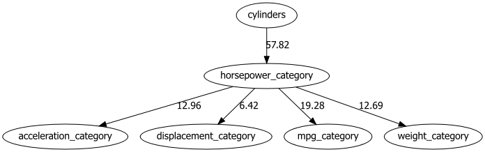

Best scoring DAG based on Hillclimbsearch and BIC scoring function for the Auto mpg dataset. All the continuous values are discretized automatically. Distfit is used to determine the 95% confidence intervals, the distribution plots are inspected and the categories are used. The edges are the -log10(Pvalues) that are determined using the chi-square test. The image is created using Bnlearn—image by the author.

3. Causal Discovery By Modelling Continuous Variables (proof of concept).

The use of discretizing methods is meaningful as it opens a broad range of Bayesian statistical methods that can be applied. However, it is not always possible or wanted to discretize the variables. There are also manners to model the continuous dataset such as with the LiNGAM method which is also implemented in Bnlearn.

The Direct-LiNGAM method is a semi-parametric approach that assumes a linear relationship among observed variables while ensuring that the error terms follow a non-Gaussian distribution, with the constraint that the graph remains acyclic. This method involves repeated regression analysis and independence assessments using linear regression with least squares. In each regression, one variable serves as the dependent variable (outcome), while the other acts as the independent variable (predictor). This process is applied to each type of variable. In other words, the lingam-direct method allows you to model continuous and mixed datasets. A disadvantage is that causal discovery of structure learning is the end-point when using this method. Thus it is not possible to perform parameter learning and probabilistic inferences.

To demonstrate its working, we will create a toy-example dataset containing six variables. The goal of this dataset is to demonstrate the contribution of different variables and their causal impact on the dependent variables. The sample size is set to n=1000 with a uniform distribution of continuous values. We will introduce dependencies between variables and then use the model to infer the original values.

Step 1: x3 is the root node and is initialized with a uniform distribution.
Step 2: x0 and x2 are created by multiplying with the values of x3, making them dependent on x3.
Step 3: x5 is created by multiplying with the values of x0, making it dependent on x0.
Step 4: x1 and x4 are created by multiplying with the values of x0, making them dependent on x0.

The experimental DAG with its causal values on the edges. The image is created using Bnlearn – image by the author.

import numpy as np
import pandas as pd
from lingam.utils import make_dot

# Number of samples
n=1000

# step 1
x3 = np.random.uniform(size=n)
# step 2
x0 = 3.0*x3 + np.random.uniform(size=n)
x2 = 6.0*x3 + np.random.uniform(size=n)
# step 3
x5 = 4.0*x0 + np.random.uniform(size=n)
# step 4
x1 = 3.0*x0 + 2.0*x2 + np.random.uniform(size=n)
x4 = 8.0*x0 - 1.0*x2 + np.random.uniform(size=n)
df = pd.DataFrame(np.array([x0, x1, x2, x3, x4, x5]).T ,columns=['x0', 'x1', 'x2', 'x3', 'x4', 'x5'])
df.head()

np.array([[0.0, 0.0, 0.0, 3.0, 0.0, 0.0],
          [3.0, 0.0, 2.0, 0.0, 0.0, 0.0],
          [0.0, 0.0, 0.0, 6.0, 0.0, 0.0],
          [0.0, 0.0, 0.0, 0.0, 0.0, 0.0],
          [8.0, 0.0,-1.0, 0.0, 0.0, 0.0],
          [4.0, 0.0, 0.0, 0.0, 0.0, 0.0]])

dot = make_dot(m)
dot

Structure learning can be applied with the direct-lingam method.

# Load library
import bnlearn as bn

# Structure learning
model = bn.structure_learning.fit(df, methodtype='direct-lingam')

# When we no look at the output, we can see that the dependency values are very well recovered for the various variables.

print(model['adjmat'])
# target        x0        x1       x2   x3        x4       x5
# source
# x0      0.000000  2.987320  0.00000  0.0  8.057757  3.99624
# x1      0.000000  0.000000  0.00000  0.0  0.000000  0.00000
# x2      0.000000  2.010043  0.00000  0.0 -0.915306  0.00000
# x3      2.971198  0.000000  5.98564  0.0 -0.704964  0.00000
# x4      0.000000  0.000000  0.00000  0.0  0.000000  0.00000
# x5      0.000000  0.000000  0.00000  0.0  0.000000  0.00000
bn.plot(model)

# Compute edge strength with the chi_square test statistic
model = bn.independence_test(model, df, prune=False)

print(model['adjmat'])
# target        x0        x1       x2   x3        x4       x5
# source
# x0      0.000000  2.987320  0.00000  0.0  8.057757  3.99624
# x1      0.000000  0.000000  0.00000  0.0  0.000000  0.00000
# x2      0.000000  2.010043  0.00000  0.0 -0.915306  0.00000
# x3      2.971198  0.000000  5.98564  0.0 -0.704964  0.00000
# x4      0.000000  0.000000  0.00000  0.0  0.000000  0.00000
# x5      0.000000  0.000000  0.00000  0.0  0.000000  0.00000

# Using the causal_order_ properties, we can see the causal ordering as a result of the causal discovery.

print(model['causal_order'])
# ['x3', 'x0', 'x5', 'x2', 'x1', 'x4']

# We can draw a causal graph by utility funciton.
bn.plot(model)

The final results are shown in the DAG below and we can see that not only the causal network is captured correctly but also the values that we intentionally used to create the causal graph in the first place.

The Estimated Causal Graph with Bnlearn very well represents the initial DAG that is created. The image is created using Bnlearn – image by the author.

3. Causal Discovery Of Continuous Datasets With The Auto MPG Dataset

As a final example, we will load the auto mpg dataset again but we will model the continuous variables without discretizing. For this approach, we will set the method to direct-lingam and then run the Structure Learning approach in bnlearn.

import bnlearn as bn

# Load example mixed dataset
df = bn.import_example(data='auto_mpg')
del df['origin']

# Structure learning or causal discovery
model = bn.structure_learning.fit(df, methodtype='direct-lingam', params_lingam = {'random_state': 2})

# Make plot
bn.plot(model)

# Compute edge strength with the chi_square test statistic
model = bn.independence_test(model, df, prune=True)

############
# Plotting #
############
bn.plot(model)
bn.plot(model, edge_labels='pvalue');

# Create interactive plot
bn.plot(model, interactive=True)

# Create graphviz plot
dotgraph = bn.plot_graphviz(model)
dotgraph
# Create pdf
dotgraph.view(filename='auto_mpg_bnlearn.pdf')

# Create graphviz plot with Pvalue on the edges
dotgraph2 = bn.plot_graphviz(model, edge_labels='pvalue')
dotgraph2

The results for causal discovery or structure learning are shown in the figure below.

Causal Discovery of the continuous auto mpg dataset using the Direct-Lingam method in Bnlearn. Figure A Depicts the weights on the edges. Figure B depicts the statistical significance between the two connected variables using the -Log10(P-value). The image is created using Bnlearn – image by the author.

Bayesian Statistics Are Great But..

So far, I've been quite enthusiastic about Bayesian approaches, but it is important to also understand some of the limitations as well. First, complex systems aren't always represented as Directed Acyclic Graphs (DAGs); some systems are cyclical, which cannot be modeled using Bayesian methods. Additionally, causal models can involve stochastic effects, meaning that repeated experiments might lead to different outcomes (local optima), even when using the same Bayesian techniques.

Then there is the Markov equivalence. This means that multiple different network structures could explain the relationships equally well using observational data alone. This makes identifying the true underlying causal structure more difficult without additional information (e.g., interventional data or domain knowledge)

Another point to keep in mind is that the results of Bayesian models can vary depending on the model used. I demonstrated with the Auto MPG data set that different modeling approaches can result in different DAGs. Criteria like BIC (Bayesian Information Criterion) often assume that simpler structures are better, which is not always true for complex systems. Always select the statistic (search method, scoring function, etc) that best fits the specific properties of your dataset and use case. The default settings of a library may not be the best settings for your use case.

Furthermore, datasets are often incomplete, either in terms of variables or insufficient sample sizes, which can also affect model outcomes. If you want to draw strong conclusions using Bayesian methods, it's important to recognize that this requires strong assumptions. In other words, building real-world applications on complex events can become troublesome, and performing independent validation tests can be required. As an example, when working on high-risk models such as modeling disease pathogenesis, one can think of performing laboratory experiments to validate the results.

Final words.

In this blog post, I showed how to apply causal discovery methods from small to large datasets. Data sets can have variables in the form of discrete, continuous, or mixed variables. I showed the application of various popular Bayesian libraries and separated supervised causal discovery approaches from unsupervised causal approaches. In the case of supervised causal approaches, libraries are designed for causal discovery using treatment and intervention variables (DoWhy, and PyMC). In the case of unsupervised causal discovery approaches, relationships can be detected from uncontrolled or observational datasets. Well-known libraries are Pgmpy, which contains low-level statistical functions, and the Bnlearn library, which contains ready-to-go pipelines, making it straightforward to detect causal relationships in small to large datasets.

Thank you for taking the time to read this guide. I hope it has provided valuable insights into applying causal discovery methods! The key to success lies in understanding which statistical methods and libraries best suit your use case. So keep experimenting with different methods, explore and compare your results, and improve your understanding of causal modeling.

Be Safe. Stay Frosty.

Cheers E.

If you found this article about Bayesian statistics useful, follow me to stay up-to-date with my latest content because I write more about this topic!

References

- Bayesian Statistics, Wikipedia
- Taskesen E. Chat with Your Dataset using Bayesian Inferences. Medium Nov. 2023
- Taskesen E, A Guide to Find the Best Boosting Model using Bayesian Hyperparameter Tuning but without Overfitting. Medium Aug. 2022
- Taskesen E, A step-by-step guide in designing knowledge-driven models using Bayesian theorem, Medium, 2021
- Taskesen E, A Step-by-Step Guide in detecting causal relationships using Bayesian Structure Learning in Python, Medium, 2021
- Kay H. et al, Inferring causal impact using Bayesian structural time-series models, 2015, Annals of Applied Statistics (247–274, vol9)
- I. A. Beinlich et al, The ALARM Monitoring System: A Case Study with Two Probabilistic Inference Techniques for Belief Networks. In Proceedings of the 2nd European Conference on Artificial Intelligence in Medicine, pages 247–256. Springer-Verlag, 1989. The data set can be found over here and is licensed under Creative Commons Attribution-Share Alike License.
- UCI Machine Learning Repository, Auto MPG dataset, licensed under a Creative Commons Attribution 4.0 International (CC BY 4.0).
- Taskesen, E. (2020). Learning Bayesian Networks with the bnlearn Python Package. (Version 0.3.22) [Computer software].
- Taskesen, E. (2020). The Power of Bayesian Causal Inference: A Comparative Analysis of Libraries to Reveal Hidden Causality in Your Dataset, Medium 2023.
- Taskesen, E (2023), Create and Explore the Landscape of Roles and Salaries in Data Science. Medium.