Back To Basics, Part Dos: Gradient Descent
Welcome to the second part of our Back To Basics series. In the first part, we covered how to use Linear Regression and Cost Function to find the best-fitting line for our house prices data. However, we also saw that testing multiple intercept values can be tedious and inefficient. In this second part, we'll delve deeper into Gradient Descent, a powerful technique that can help us find the perfect intercept and optimize our model. We'll explore the math behind it and see how it can be applied to our linear regression problem.
Gradient descent is a powerful optimization algorithm that aims to quickly and efficiently find the minimum point of a curve. The best way to visualize this process is to imagine you are standing at the top of a hill, with a treasure chest filled with gold waiting for you in the valley.

However, the exact location of the valley is unknown because it's super dark out and you can't see anything. Moreover, you want to reach the valley before anyone else does (because you want all of the treasure for yourself duh). Gradient descent helps you navigate the terrain and reach this optimal point efficiently and quickly. At each point, it'll tell you how many steps to take and in what direction you need to take them.
Similarly, gradient descent can be applied to our Linear Regression problem by using the steps laid out by the algorithm. To visualize the process of finding the minimum, let's plot the MSE curve. We already know that the equation of the curve is:

And from the previous article, we know that the equation of MSE in our problem is:

If we zoom out we can see that an MSE curve (which resembles our valley) can be found by substituting a bunch of intercept values in the above equation. So let's plug in 10,000 values of the intercept, to get a curve that looks like this:

The goal is to reach the bottom of this MSE curve, which we can do by following these steps:
Step 1: Start with a random initial guess for the intercept value
In this case, let's assume our initial guess for the intercept value is 0.
Step 2: Calculate the gradient of the MSE curve at this point
The gradient of a curve at a point is represented by the tangent line (a fancy way of saying that the line touches the curve only at that point) at that point. For example, at Point A, the gradient of the MSE __ curve can be represented by the red tangent line, when the intercept is equal to 0.

In order to determine the value of the gradient, we apply our knowledge of calculus. Specifically, the gradient is equal to the derivative of the curve with respect to the intercept at a given point. This is denoted as:

NOTE: If you're unfamiliar with derivatives, I recommend watching this Khan Academy video if interested. Otherwise you can gloss over the next part and still be able to follow the rest of the article.
We calculate the derivative of the MSE curve as follows:

Now to find the gradient at point A, we substitute the value of the intercept at point A in the above equation. Since intercept = 0, the derivative at point A is:

So when the intercept = 0, the gradient = -190
NOTE: As we approach the optimal value, the gradient values approach zero. At the optimal value, the gradient is equal to zero. Conversely, the farther away we are from the optimal value, the larger the gradient becomes.
From this, we can infer that the step size should be related to the gradient since it tells us if we should take a baby step or a big step. This means that when the gradient of the curve is close to 0, then we should take baby steps because we are close to the optimal value. And if the gradient is bigger, we should take bigger steps to get to the optimal value faster.
NOTE: However, if we take a super huge step, then we could make a big jump and miss the optimal point. So we need to be careful.

Step 3: Calculate the Step Size using the gradient and the Learning Rate and update the intercept value
Since we see that the Step Size and gradient are proportional to each other, the Step Size is determined by multiplying the gradient by a pre-determined constant value called the Learning Rate:

The Learning Rate controls the magnitude of the Step Size and ensures that the step taken is not too large or too small.
In practice, the Learning Rate is usually a small positive number that is ≤ 0.001. But for our problem let's set it to 0.1.
So when the intercept is 0:

Based on the Step Size we calculated above, we update the intercept (aka change our current location) __ using any of these equivalent formulas:

To find the new intercept in this step, we plug in the relevant values…

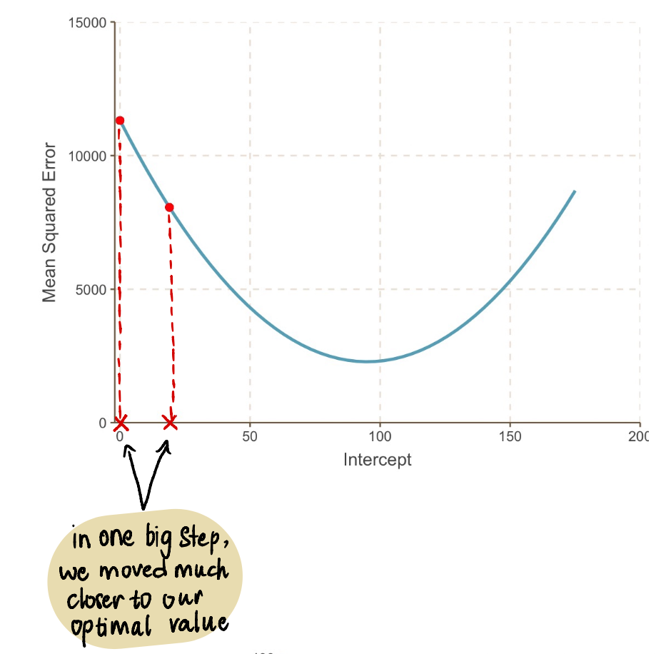
…and find that the new intercept = 19.
Now plugging this value in the MSE equation, we find that the MSE when the intercept is 19 = 8064.095. In one big step, we moved closer to our optimal value and reduced the MSE.
Even if we look at our graph, we see how much better our new line with intercept 19 is fitting our data than our old line with intercept 0:

Step 4: Repeat steps 2–3
We repeat Steps 2 and 3 using the updated intercept value.
For example, since the new intercept value in this iteration is 19, following Step 2, we will calculate the gradient at this new point:

And we find that the gradient of the MSE curve at the intercept value of 19 is -152 (as represented by the red tangent line in the illustration below).

Next, in accordance with Step 3, let's calculate the Step Size:

And subsequently, update the intercept value:

Now we can compare the line with the previous intercept of 19 to the new line with the new intercept 34.2…

…and we can see that the new line fits the data better.
Overall, the MSE is getting smaller…

…and our Step Sizes are getting smaller:

We repeat this process iteratively until we converge toward the optimal solution:

As we progress toward the minimum point of the curve, we observe that the Step Size becomes increasingly smaller. After 13 steps, the gradient descent algorithm estimates the intercept value to be 95. If we had a crystal ball, this would be confirmed as the minimum point of the MSE curve. And it is clear to see how this method is more efficient compared to the brute force approach that we saw in the previous article.
Now that we have the optimal value of our intercept, the linear regression model is:

And the linear regression line looks like this:

Finally, going back to our friend Mark's question – What value should he sell his 2400 feet² house for?

Plug in the house size of 2400 feet² into the above equation…

…and voila. We can tell our unnecessarily worried friend Mark that based on the 3 houses in his neighborhood, he should look to sell his house for around $260,600.
Now that we have a solid understanding of the concepts, let's do a quick Q&A sesh answering any lingering questions.
Why does finding the gradient actually work?
To illustrate this, consider a scenario where we are attempting to reach the minimum point of curve C, denoted as x*. And we are currently at point A at x, located to the left of x*:
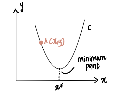
If we take the derivative of the curve at point A with respect to x, represented as dC(x)/dx, we obtain a negative value (this means the gradient is sloping downwards). We also observe that we need to move to the right to reach x*. Thus, we need to increase x to arrive at the minimum x*.

Since dC(x)/dx is negative, x-
