Building a Convolutional Neural Network (CNNs) from Scratch
One of the reasons Machine Learning is such an interesting field is it allows us to apply computing logic to areas that previously were untouchable. While computers are extremely effective with arrays and integers, they have traditionally been less apt at dealing with emergent properties. For example, you cannot look at just one pixel on a screen and know the image is a dog. You have to synthesize lots of data points.
In the past decade, computer scientists were able to bridge this divide by creating Computer Vision models— specifically Convolutional Neural Networks (CNNs). Today, I'm going to show how to apply them to image classification.
Classification of real world data is very useful for integrating machine learning technology into more typical software systems. If you're in e-commerce, you may use this information to automatically categorize a new product. If you're in medicine, you may use this to determine if an X-Ray or MRI looks similar to previous images that required surgery. Finally, if you're in a vehicle and looking to drive safely, image classification is a key part of object detection and collision avoidance.
Let's dive in!
Parts of Convolutional Neural Networks
Convolution
Let's start off by explaining what a convolution is. In mathematics, a convolution is a way of taking two sets, applying an operation on both and creating a third set. The reason we use this in image models is because our data fits nicely into this formula. For example, an initial convolution would have set one as our input image, set two as the weights we've trained our model to have, and set three as the output to the next layer.

Convolutions typically change the input along the depth dimension (channels), while spatial dimensions (x,y) are left untouched when proper padding is applied. To understand this better, let's explore an example of an image with dimensions (width_x, width_y, 3). Width_x is the width of our image, width_y is our height, and 3 represents each of our color channels: 1 for Red, 1 for Green, 1 for Blue (RGB format).
Now if we perform a convolution on these color channels with a set of depth 64, we will then create an output of 64. This results in the output dimensions now changing from (width_x, width_y, 3) to (width_x, width_y, 64). This works if the depth channel is bigger or smaller than the input.
Non-Linearity
While a lot of data is good, not all data is created equal. Therefore, we do not want our model to pay equal attention to all of the data it's processing. In neural networks, a neuron fires when data should be passed through. Similar to the Transformer architecture, CNNs use non-linear activation functions to determine which neurons should fire. These functions are often the same such as GeLU and ReLU.

Pooling
Pooling is not typically seen in Transformer architectures, though it is critical in CNNs. In addition to using non-linearity to determine which neurons fire, we use pooling layers to reduce the amount of information that is brought through. The balance here is to reduce the dimensionality of data while not losing signal regarding key features.

Batch Normalization
This function is a way to "stabilize" our learnings. The basic idea is to assume that the neuron activations will largely follow a normal distribution, and thus we can use Gaussian methodologies to have the activation distribution fit to a normal curve. By fitting to this curve, you reduce the odds that one piece of data is given a massive activation and thus ends up throwing the entire model down the wrong path.
See more about batch normalization with this excellent blog.
Major Open Source Image Models
Now that we have the vocabulary, let's examine a few of the major image models to see how these concepts come together.
VGG
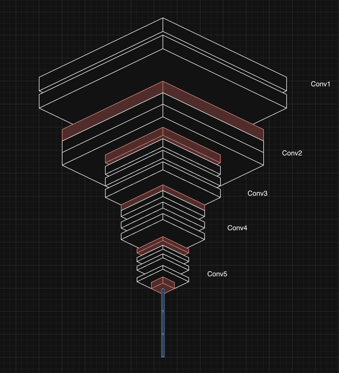
Visual Geometry Group (VGG) was one of the first major models to achieve high-quality accuracy on a major image data set (ImageNet). VGG is simpler than many other architectures today – mainly focusing on spatial hierarchies (think position within an image) as oppose to temporal or frequency-based approaches. You can see in the above that we have multiple convolution layers which get their spatial dimensions reduced by the pool layers (shown in red). Finally, at the very end we have a series of linear layers that will give us the final classification.
ResNet
ResNet was created by Microsoft [2] also as part of the ImageNet competition. This model's major insight was around training deeper models (models with more layers within). Before ResNet, there were issues with vanishing gradients. Because each layer needs a gradient dependent on the input from the last, having so many gradients would eventually lead to no updates happening on earlier layers. Consequently, the performance would be terrible – it was as if you were only training a small portion of your model.
Microsoft fixed this by adding in a residual – a part of the previous layer's input that will be processed to create the next layer's output. This passes information to the next layer directly allowing the gradients from previous layers to pass through information even if their gradients are inconsequential. Thus, more weights get updated and we avoid vanishing gradients.

Comparing Architectures
ResNet is newer than VGG and also happens to be very common. Comparing the two architectures on a separate dataset [3], it looks like ResNet is more accurate, so I'll go with this one.
Training Dataset

Now that we have our base model, we need a good dataset to train on. The mnist-fashion dataset is used often in this space as it's MIT licensed, openly available, and has a significant number of data (60k images in total).
Like any good data scientist, we need to understand our data before we begin training on it. Looking through the entries, we see that our data consists of an equal number of 10 classes of data (t-shirt, trouser, pullover, dress, coat, sandal, shirt, sneaker, bag, ankle boot), where each image is 28 x 28 pixels. Because the images are in grayscale, we have only 1 color channel.
Code
Now that we understand the theory and the data we're training on, let's start coding up an implementation!
Before I begin, I want to give credit to the Jovian team, whose excellent PyTorch tutorial heavily inspired the below code.
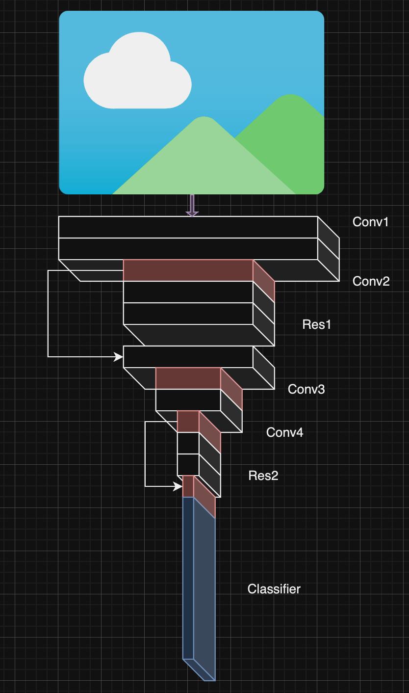
ResNet9
Given the relatively low resolution of our MNIST-Fashion dataset, we're going to have fewer pooling operations in our model. This is because every time you do a pooling operation, you are reducing the spatial dimensions further. With an initial image size of just 28 pixels, you can effectively over-process the image, resulting in the last layers of our model not getting sufficient signal.
Let's dive into how we encode this in PyTorch:
class ResNet9(nn.Module):
    def __init__(self, in_channels, num_classes):
        super().__init__()

        self.conv1 = self.conv_block(in_channels, 64)
        self.conv2 = self.conv_block(64, 128, pool=True)
        self.res1 = nn.Sequential(self.conv_block(128, 128), self.conv_block(128, 128))

        self.conv3 = self.conv_block(128, 256, pool=True)
        self.conv4 = self.conv_block(256, 512, pool=True)
        self.res2 = nn.Sequential(self.conv_block(512, 512), self.conv_block(512, 512))

        self.classifier = nn.Sequential(nn.MaxPool2d(3),
                                        nn.Flatten(),
                                        nn.Linear(512, num_classes))

    def training_step(self, batch):
        images, labels = batch
        out = self(images)
        loss = F.cross_entropy(out, labels)
        return loss

    def validation_step(self, batch):
        images, labels = batch
        out = self(images)
        loss = F.cross_entropy(out, labels)
        acc = accuracy(out, labels)
        return {'val_loss': loss.detach(), 'val_acc': acc}

    def validation_epoch_end(self, outputs):
        batch_losses = [x['val_loss'] for x in outputs]
        epoch_loss = torch.stack(batch_losses).mean()
        batch_accs = [x['val_acc'] for x in outputs]
        epoch_acc = torch.stack(batch_accs).mean()
        return {'val_loss': epoch_loss.item(), 'val_acc': epoch_acc.item()}

    def epoch_end(self, epoch, result):
        print("Epoch [{}], last_lr: {:.5f}, train_loss: {:.4f}, val_loss: {:.4f}, val_acc: {:.4f}".format(
            epoch, result['lrs'][-1], result['train_loss'], result['val_loss'], result['val_acc']))

    def conv_block(self, in_channels, out_channels, pool=False):
        layers = [nn.Conv2d(in_channels, out_channels, kernel_size=3, padding=1),
                nn.BatchNorm2d(out_channels),
                nn.ReLU(inplace=True)]
        if pool:
            layers.append(nn.MaxPool2d(2))
        return nn.Sequential(*layers)

    def forward(self, xb):
        out = self.conv1(xb)
        out = self.conv2(out)
        out = self.res1(out) + out
        out = self.conv3(out)
        out = self.conv4(out)
        out = self.res2(out) + out
        out = self.classifier(out)
        return out
Let's dive into 2 of the functions above: conv_block and forward.
conv_block is defining what we do for each convolution in our model. We have either 3 or 4 layers based off where this block is within the model. Every convolution block will use a two dimensional convolution where the kernel will always be 3×3 and have a padding of 1. Once that's complete, we'll do a batch normalization to stabilize our activations. Finally, we'll use the ReLU function to activate only certain neurons going forwards. The inplace parameter tells us that we are modifying the input tensor directly (this is a memory optimization). Finally, if we want to have a pooling operation here, we will use a MaxPool with a kernel size of 2×2 – thus reducing our spatial dimensions by 50%.
forwardtells the model how to do a forward pass, so here we encode the ResNet architecture. We go through 4 convolution blocks (1 in conv1, 1 in conv2, and 2 in res1) and then add back the output from conv2 to the output of res1. When people talk about residual networks, it is this operation they are talking about. We repeat that pattern again and then pass the output to our linear layer at the end to give us back our classifications.
Note, our maxpool operation in the classifier is the largest size possible to process the image at that point. Going through each stage, we begin with data of dimensions (28x28x1), then we go to (28x28x64), then (14x14x128), then (14x14x128), then (7x7x256), then (3x3x512). Our classifier at the end processes with a 3×3 kernel, which is the largest our (3x3x512) data can handle.
Data Loader
The data loader is necessary to ensure our data is always in the right place. PyTorch wants us to specify which device certain data should reside on. To ensure our data is always where we need it, we'll use the DeviceDataLoader to ensure that every batch is moved to the right device for processing. We also have a function to clear the cache for our device and to let us know which device we have access to. We setup a hierarchy of devices to use. If CUDA is available, we'll always use that. If not, then we will check if Apple Silicon is available and then we default to CPU.
import torch

def get_default_device():
    """Pick GPU if available, else CPU"""
    if torch.cuda.is_available():
        return torch.device("cuda")
    elif torch.backends.mps.is_available():
        return torch.device("mps")
    else:
        return torch.device("cpu")

def clear_cache():
    if torch.cuda.is_available():
        torch.cuda.empty_cache()
    elif torch.backends.mps.is_available():
        torch.mps.empty_cache()

def to_device(data, device):
    """Move tensor(s) to chosen device"""
    if isinstance(data, (list,tuple)):
        return [to_device(x, device) for x in data]
    return data.to(device, non_blocking=True)

class DeviceDataLoader():
    """Wrap a dataloader to move data to a device"""
    def __init__(self, dl, device):
        self.dl = dl
        self.device = device

    def __iter__(self):
        """Yield a batch of data after moving it to device"""
        for b in self.dl:
            yield to_device(b, self.device)

    def __len__(self):
        """Number of batches"""
        return len(self.dl)

device = get_default_device()
print(f"running on {device}")
Training Loop
This is the function where most of our compute is going to go, so let's dive deep. We begin by emptying our cache to ensure that we aren't having any unnecessary data in memory. Next, we setup our optimizer and scheduler.
The optimizer calculates gradients and performs backpropagation to update the model's weights after each batch. We have different strategies for finding gradients such as Adam, AdamW, Stochastic Gradient Descent, and more. While we are setting the default to SGD, I've found that AdamW outdoes Adam and SGD on this specific setup (more on this later).
The scheduler is in charge of picking out what our learning rate should be for a specific epoch. The learning rate is the epsilon that our gradients are multiplied by to update the rates. You can imagine something like Wn += Gradient * Lr. Thus, the higher the learning rate, the more dramatically the model changes. Over time, researchers have seen that varying the learning rate throughout the training run produces the best results. This typically follows the pattern of higher learning rates at the beginning and lower ones towards the end. We are using OneCycleLR, which will spend 30% of the training increasing the learning rate up to our set maximum, and then slowly scale down to zero by the end.
def get_lr(optimizer):
    for param_group in optimizer.param_groups:
        return param_group['lr']

def fit_one_cycle(epochs, max_lr, model, train_loader, val_loader,
                  weight_decay=0, grad_clip=None, opt_func):
    clear_cache()
    history = []

    optimizer = opt_func(model.parameters(), max_lr, weight_decay=weight_decay)
    sched = torch.optim.lr_scheduler.OneCycleLR(optimizer, max_lr, epochs=epochs,
                                                steps_per_epoch=len(train_loader),
                                                pct_start=0.3)

    for epoch in range(epochs):
        model.train()
        train_losses = []
        lrs = []
        for batch in train_loader:
            loss = model.training_step(batch)
            train_losses.append(loss)
            loss.backward()

            if grad_clip:
                nn.utils.clip_grad_value_(model.parameters(), grad_clip)

            optimizer.step()
            optimizer.zero_grad()

            lrs.append(get_lr(optimizer))
            sched.step()

        result = evaluate(model, val_loader)
        result['train_loss'] = torch.stack(train_losses).mean().item()
        result['lrs'] = lrs
        model.epoch_end(epoch, result)
        history.append(result)
    return history
After we train, we want to get a sense of how well our model is now doing. We use the validation training set here after every epoch to benchmark. We'll use the validation data for two things: gauging overfitting and performance. If we see validation accuracy stagnates while training accuracy goes up, this suggests we are overfitting. In this case, training loss would continue to decrease while validation loss remains constant. Conversely, if validation and training loss continue going down together, then we can infer that signal is still being trained and we are good to train for more epochs. Finally, if both training and validation metrics plateau, then we can infer we're reaching the limit of our data or architecture (this was the point where the authors of ResNet began their work).
Validation
Validation and inferencing the finished model will look practically identical. We start by telling torch not to store any gradients as we won't need any backpropagation. We then set the model into eval mode & finally run the model on the validation set in batches. Note, we are running validation on the entire validation set every time. This ensures consistent comparisons between epochs.
@torch.no_grad()
def evaluate(model, val_loader):
    model.eval()
    outputs = [model.validation_step(batch) for batch in val_loader]
    return model.validation_epoch_end(outputs)
Data Augmentation
To improve accuracy, we typically look to augment our data in some way. This helps for two reasons. First, we have more variety in the data we're training on, so the model sees more of the imperfection it's likely to experience in the real world. Second, by adding these variations into the training set, we also have more data for it to train on.
We need to strike a balance when augmenting so the features of the original images remain for the model to learn. A good rule of thumb is if you have no idea what the image is, then likely the model will struggle.
basic_tfms = tt.Compose([tt.ToTensor(), tt.Normalize(*stats)])
train_fms = tt.Compose([tt.RandomCrop(28, padding=4, padding_mode='reflect'),
tt.RandomHorizontalFlip(p=0.5),
tt.RandomVerticalFlip(p=0.5),
tt.ToTensor(),
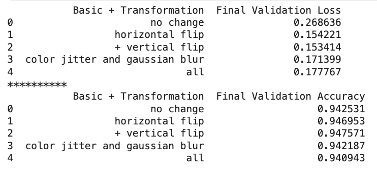
tt.Normalize(*stats,inplace=True)])In my case, I found having 2 sets of training data gave the best accuracy: one with minimal changes and one where images were randomly flipped horizontally and vertically. See the code I wrote to compare data augmentations here.

Hyperparameters
Finally, below are the hyperparameters I chose. I did another quick ablation study to pick what these should be based off the highest accuracy. I selected the parameter ranges through systematic testing, beginning with epochs, followed by learning rate, weight decay, and then the optimizer function.
epochs = 16
max_lr = 0.007
grad_clip = 0.1
weight_decay = 1e-4
opt_func = torch.optim.AdamW
See the code I wrote to compare hyperparameters here.
Training Results


After training on the above hyperparameters I found that our model reached 94.8% accuracy typically, though other runs could reach into 95%. Going from the graphs above, we can see some things that we may want to improve for next time. Most interestingly, it looks like the training and loss rates plateaued at the roughly same time. This suggests that we may be at the limit of our current architecture to improve performance. Some places that are worth looking into are to increase the channel size in the middle of the model, adjusting our scheduler to use cosine annealing, and adding a warmup period for the first batch.
Closing
In closing, CNNs are an incredibly powerful type of machine learning. We went through and trained one from scratch on the MNIST-Fashion dataset. When you apply these models to more areas, you will want to revisit which architecture is best, how you should modify it, and what data you have at your disposal.
To check out all the Jupyter Notebooks I used for training, you can go to the Github link below.
It's an exciting time to be building!
[1] Rao, A., "Classifying CIFAR10 images using ResNets, Regularization and Data Augmentation in PyTorch" (2021), Jovian
[2] He, K., et al., "Deep Residual Learning for Image Recognition" (2015), arXiv
[3] Anwar, A., "Difference between AlexNet, VGGNet, ResNet, and Inception" (2019), Towards Data Science
