Building PCA from the Ground Up

Principal Component Analysis (PCA) is an old technique commonly used for dimensionality reduction. Despite being a well-known topic among data scientists, the derivation of PCA is often overlooked, leaving behind valuable insights about the nature of data and the relationship between calculus, statistics, and linear algebra.
In this article, we will derive PCA through a thought experiment, beginning with two dimensions and extending to arbitrary dimensions. As we progress through each derivation, we will see the harmonious interplay of seemingly distinct branches of mathematics, culminating in an elegant coordinate transformation. This derivation will unravel the mechanics of PCA and reveal the captivating interconnectedness of mathematical concepts. Let's embark on this enlightening exploration of PCA and its beauty.
Warming Up in Two Dimensions
As humans living in a three-dimensional world, we generally grasp two-dimensional concepts, and this is where we will begin in this article. Starting in two dimensions will simplify our first thought experiment and allow us to better understand the nature of the problem.
Theory
We have a dataset that looks something like this (note that each feature should be scaled to have a mean of 0 and variance of 1):

We immediately notice this data lies in a coordinate system described by x1 and x2, and these variables are correlated. Our goal is to find a new coordinate system informed by the covariance structure of the data. In particular, the first basis vector in the coordinate system should explain the majority of the variance when projecting the original data onto it.
Our first order of business is to find a vector such that when we project the original data onto the vector, the maximum amount of variance is preserved. In other words, the ideal vector points in the direction of maximal variance, as defined by the data.
This vector can be defined by the angle it makes with the x-axis in the counter-clockwise direction:

In the animation above, we define a vector by the angle it makes with the x- axis, and we can see the direction the vector points at each angle between 0 and 180 degrees. Visually, we can see that a θ value near 45 degrees points in the direction of maximal variability in the data.
To restate our objective, we want to find the angle the causes the vector to point in the direction of maximal variance. Mathematically, we want to find θ that maximizes this equation:

Here, N is the number of observations in the data. We project each observation onto the axis defined by [cos(θ) sin(θ)], which is a unit vector defined by the angle θ, and square the result.
As we vary θ, this equation gives of the variance of the data when projected onto the axis defined by θ. Let's compute the dot product inside the square and rewrite this expression to make it easier to work with:

Luckily for us, this is a convex function, and we can maximize it by computing it's derivative and setting it equal to 0. We will also need to compute the second derivative of the variance equation to know whether we've found a minima or maxima. The first and second derivatives of var(θ) look like this:

Next, we can set the first derivative equal to 0, and rearrange the equation to isolate θ:

Finally, using a common trig identity and some algebra, we get a closed form solution for the θ that minimizes or maximizes var(θ):

Fascinatingly, this equation is all we need to perform PCA in two dimensions. The second derivative will tell us whether θ corresponds to a local minima or maxima. Because there is only one other principal component, it must be defined by shifting θ by 90 degrees. Therefore, the two principal component angles are given by:

As mentioned before, we can use the second derivative of var(θ) to figure out which θ belongs to principal component 1 (the direction of maximal variance) and which θ belongs to principal component 2 (the direction of minimal variance). Alternatively, we can plug both θs into var(θ) and see which one results in a higher value.
Once we know which θ corresponds to each principal component, we plug each one into the trigonometric equation for a unit vector in two dimensions ([cos(θ) sin(θ)]). Explicitly, we do the following:

That's it – pc1 and pc2 are the principal component vectors. By thinking through the objective of principal component analysis, we were able to derive the principal components from scratch in two dimensions. To convince ourselves this is correct, let's write some Python code to implement our strategy.
Code
The first function finds one of the principal angles derived from the derivative of the variance equation in figure (7). Because this is a closed-form equation, the implementation is straight forward:
import numpy as np

def find_principal_angle(x1: np.ndarray, x2: np.ndarray) -> float:
    """
    Find the angle corresponding to one of the principal components
    in two dimensions.

    Parameters
    ----------
    x1 : numpy.ndarray
        First input vector with shape (n,).
    x2 : numpy.ndarray
        Second input vector with shape (n,).

    Returns
    -------
    float
        The principal angle in radians.
    """

    cov = -2 * np.sum(x1 * x2)
    var_diff = np.sum(x2**2 - x1**2)

    return 0.5 * np.arctan(cov / var_diff)
Depending on the nature of the variance equation, find_principal_angle() recovers one of the principal angles, and the other principal angle is 90 degrees away. To determine which principal angle find_principal_angle() returns, we can use the second derivative, or hessian, of the variance equation:
def compute_pca_cost_hessian(x1: np.ndarray,
                             x2: np.ndarray,
                             theta: float) -> float:
    """
    Compute the Hessian of the cost function for Principal Component
    Analysis (PCA) in two dimensions.

    Parameters
    ----------
    x1 : numpy.ndarray
        First input vector with shape (n,).
    x2 : numpy.ndarray
        Second input vector with shape (n,).
    theta : float
        An angle in radians for which the cost function is evaluated.

    Returns
    -------
    float
        The Hessian of the PCA cost function evaluated at the given theta.
    """

    return np.sum(
        2 * (x2**2 - x1**2) * np.cos(2 * theta) -
        4 * x1 * x2 * np.sin(2 * theta)
    )
The logic for this function comes directly from figure (5). The last function we need determines the two principal components from find_principal_angle() and compute_pca_cost_hessian():
def find_principal_components_2d(x1: np.ndarray, x2: np.ndarray) -> tuple:
    """
    Find the principal components of a two-dimensional dataset.

    Parameters
    ----------
    x1 : numpy.ndarray
        First input vector with shape (n,).
    x2 : numpy.ndarray
        Second input vector with shape (n,).

    Returns
    -------
    tuple
        A tuple containing the two principal components represented as
        numpy arrays.
    """

    theta0 = find_principal_angle(x1, x2)
    theta0_hessian = compute_pca_cost_hessian(x1, x2, theta0)

    if theta0_hessian > 0:
        pc1 = np.array([np.cos(theta0 + (np.pi / 2)),
                        np.sin(theta0 + (np.pi / 2))])
        pc2 = np.array([np.cos(theta0), np.sin(theta0)])
    else:
        pc1 = np.array([np.cos(theta0), np.sin(theta0)])
        pc2 = np.array([np.cos(theta0 + (np.pi / 2)),
              np.sin(theta0 + (np.pi / 2))])

    return pc1, pc2
In find_principal_components_2d(), theta0is one of the principal angles and theta0_hessianis the second derivative of the variance equation. Because theta0is an extrema of the variance equation, theta0_hessiantells us whether theta0is a minimum or maximum. In particular, if theta0_hessianis positive, theta0must be a minimum and correspond to the second principal component. Otherwise, theta0_hessianis negative and theta0is a maximum corresponding to the first principal component.
To verify find_principal_components_2d()does what we want, let's find the principal components for a two dimensional dataset and compare them to the results of the PCA implementation in scikit-learn. Here's the code:
import numpy as np
from sklearn.decomposition import PCA

# Generate two random correlated arrays
rng = np.random.default_rng(seed=80)
x1 = rng.normal(size=1000)
x2 = x1 + rng.normal(size=len(x1))

# Normalize the data
x1 = (x1 - x1.mean()) / x1.std()
x2 = (x2 - x2.mean()) / x2.std()

# Find the principal components using the 2D logic
pc1, pc2 = find_principal_components_2d(x1, x2)

# Find the principal components using sklearn PCA
model = PCA(n_components=2)
model.fit(np.array([x1, x2]).T)
pc1_sklearn = model.components_[0, :]
pc2_sklearn = model.components_[1, :]

print(f"Derived PC1: {pc1}")
print(f"Sklearn PC1: {pc1_sklearn} n")
print(f"Derived PC2: {pc2}")
print(f"Sklearn PC2: {pc2_sklearn}")

"""
Derived PC1: [0.70710678 0.70710678]
Sklearn PC1: [0.70710678 0.70710678]

Derived PC2: [ 0.70710678 -0.70710678]
Sklearn PC2: [ 0.70710678 -0.70710678]
"""

# Visualize the results
fig, ax = plt.subplots(figsize=(10, 6))
ax.scatter(x1, x2, alpha=0.5)
ax.quiver(0, 0, pc1[0], pc1[1],  scale_units='xy', scale=1, color='red')
ax.quiver(0, 0, pc2[0], pc2[1],  scale_units='xy', scale=1, color='red', label="Custom PCs")
ax.quiver(0, 0, pc1_sklearn[0], pc1_sklearn[1],  scale_units='xy', scale=1, color='green')
ax.quiver(0, 0, pc2_sklearn[0], pc2_sklearn[1],  scale_units='xy', scale=1, color='green', label="Sklearn PCs")
ax.set_xlabel("$x_1$")
ax.set_ylabel("$x_2$")
ax.set_title("Custom 2D PCA vs Sklearn PCA")
ax.legend()
This code creates two-dimensional correlated data, normalizes it, and finds the principal components using our custom logic and the scikit-learn PCA implementation. We can see that we've achieved the exact same results as scikit-learn. The resulting principal components look like this:

As expected, the two sets of principal components perfectly overlap. However, the issue with our method is that it doesn't generalize beyond two dimensions. In the next section, we will derive an analogous results for arbitrary dimensions.
Deriving a General Result
In two dimensions, we derived a closed form equation to find the principal components using the definition of variance, calculus, and a bit of trigonometry. Unfortunately, this approach will quickly become infeasible for datasets beyond two dimensions. For this, we will have to rely on the most powerful branch of mathematics for computation – linear algebra.
Theory
The derivation of PCA in higher dimensions is analogous to the two-dimensional case in many ways. The fundamental difference is that we have to leverage some tools from linear algebra to help us account for all possible angles that the principal components can make with the origin of the data.
To start, assume our data set has d features and n observations. As before, each feature should be scaled to have a mean of 0 and variance of 1. We will arrange the data in a matrix as follows:

As before, our goal is to find a unit vector, p, that points in the direction of maximum variance of the data. To do this we first need to state two useful facts. The first is that the covariance matrix of our data, the analog of variance in higher dimensions, can be found my a multiplying X with its transpose:

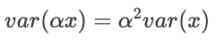
While this is useful, we're not interested in the variance of the data itself. We want to know the variance of the data when projected onto a new axis. To do this, we recall a result about the variance of a scalar quantity. Namely, when a scalar is multiplied by a constant, the resulting variance is that constant squared multiplied by the original variance:
Analogously, when we multiply a vector with our data matrix (i.e. when we project a vector onto the matrix), the resulting variance can be computed as follows:

This gives us everything we need to define our problem for PCA. That is, we want to find the vector p (the principal component) that maximizes the following equation:

The PCA problem statement in d dimensions is to find the vector, p, that maximizes the variance when projected onto the data. We also stipulate that p is a unit vector, making this a constrained optimization problem. Therefore, just as in the two-dimensional case, we need calculus.
To solve this, we can leverage lagrange multipliers, which allow us to minimize the objective while still meeting the specified constraints. The Lagrangian expression for this problem is given by:

To optimize this, we take the derivative and set it equal to 0:

Some rearranging gives us the following expression – a very familiar result from linear algebra:

What does this tell us? Astonishingly, the optimal principal component (p), when multiplied by the covariance matrix of data (S), is simply that same p multiplied by a scalar (λ). In other words, p must be an eigenvector of the covariance matrix, and we can find p by computing the eigenvalue decomposition of S. We also observe:
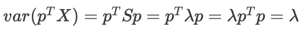
The variance of the data when projected onto p is equal to the eigenvalue corresponding to p. We also know that **** there are at most d eigenvalues/eigenvectors of S, the eigenvectors are orthogonal, and the eigenvalues are sorted from largest to smallest. This means, by taking the eigenvalue decomposition of S, we recover all of the principal components:

This is quite a beautiful intersection of statistics, calculus, and linear algebra, giving us an elegant way to find the principal components of high dimensional datasets. What a beautiful result!
Code
If we use NumPy, the general form of PCA is actually easier to code than the two-dimensional version we derived. Here's an example of PCA using a three-dimensional dataset:
import numpy as np
from sklearn.decomposition import PCA

# Generate three random correlated arrays
rng = np.random.default_rng(seed=3)
x1 = rng.normal(size=1000)
x2 = x1 + rng.normal(size=len(x1))
x3 = x1 + x2 + rng.normal(size=len(x1))

# Create the data matrix (X)
X = np.array([x1, x2, x3]).T

# Normalize X
X = (X - X.mean(axis=0)) / X.std(axis=0)

# Compute the covariance matrix of X (S)
S = np.cov(X.T)

# Compute the eigenvalue decomposition of S
variances, pcs_derived = np.linalg.eig(S)

# Sort the pcs according to their variance
sorted_idx = np.argsort(variances)[::-1]
pcs_derived = pcs_derived.T[sorted_idx, :]

# Find the pcs using sklearn PCA
model = PCA(n_components=3)
model.fit(X)
pcs_sklearn = model.components_

# Compute the element-wise difference between the pcs
pc_diff = np.round(pcs_derived - pcs_sklearn, 10)

print("Derived Principal Components: n", pcs_derived)
print("Sklearn Principal Components: n", pcs_derived)
print("Difference: n", pc_diff)

"""
Derived Principal Components:
 [[-0.56530668 -0.57124206 -0.59507215]
 [-0.74248305  0.66666719  0.06537407]
 [-0.35937066 -0.47878738  0.80100897]]
Sklearn Principal Components:
 [[-0.56530668 -0.57124206 -0.59507215]
 [-0.74248305  0.66666719  0.06537407]
 [-0.35937066 -0.47878738  0.80100897]]
Difference:
 [[ 0.  0.  0.]
 [ 0.  0. -0.]
 [ 0.  0.  0.]]
"""
As we can see, the principal components given by the scikit-learn PCA implementation are exactly the eigenvectors of the covariance matrix.
Final Thoughts
Principal Component Analysis (PCA) is a powerful technique used in Data Science and machine learning to reduce the dimensionality of high-dimensional datasets while preserving the most important information. In this article, we explored the foundational principles of PCA in two dimensions and extended it to arbitrary dimensions using linear algebra.
In the two-dimensional case, we derived a closed-form solution for finding the principal components by maximizing the variance when the data is projected onto a new axis. We used trigonometry and calculus to find the angles that define the principal components. We then implemented our strategy in Python and verified its correctness by comparing the results to the scikit-learn PCA implementation.
Moving to arbitrary dimensions, we leveraged linear algebra to find a generalized solution. By expressing PCA as an eigenvalue problem, we showed that the principal components are the eigenvectors of the covariance matrix. The corresponding eigenvalues represent the variance of the data when projected onto each principal component.
As we often see in Mathematics, seemingly unrelated concepts that were developed by different mathematicians over varying time periods end up culminating into a beautiful result. PCA is a prime example of this perplexing intersection, and there are many more to be explored!
Become a Member: https://harrisonfhoffman.medium.com/membership
Buy me a coffee: https://www.buymeacoffee.com/HarrisonfhU
References
- Ali Ghodsi, Lec 1: Principal Component Analysis – https://www.youtube.com/watch?v=L-pQtGm3VS8&t=3129s
- Independent Component Analysis 2 – https://www.youtube.com/watch?v=olKgmOuAvrc
