Causal Inference with Python: A Guide to Propensity Score Matching

Evaluating the impact of treatments or interventions is critical in various fields, both in commercial and public settings. Determining whether a specific action produces the desired effect is essential for making informed decisions. While randomized experiments are considered the gold standard for such evaluations, they are not always feasible.
Various Causal Inference methods can be utilized to estimate treatment effects in these cases. This article describes the powerful method used in the causal inference workshop: propensity score matching, providing a guide to this analytical technique.
What is Propensity Score Matching?
Propensity score matching (PSM) allows us to construct an artificial control group based on the similarity of the treated and non-treated individuals. When applying PSM, we match each treated unit with a non-treated unit of similar characteristics.
This way, we can obtain a control group without the randomized experiment. This artificial control group would consist of the non-treated units that resemble the treated group as much as possible.
While the concept of PSM may seem straightforward, its successful implementation is often complex. The key challenge lies in the details of the method, particularly in finding suitable matches based on the available data and each unit's pre-treatment characteristics.
Evaluating the Job Training Program
To explore propensity score matching, we will use the Lalonde dataset. The dataset originates from a study by Robert LaLonde (1986), which aimed to assess the effectiveness of a job training program on earnings. We will use the dataset used by Dehejia and Wahba in their paper "Causal Effects in Non-Experimental Studies: Reevaluating the Evaluation of Training Programs."
The study evaluates the National Supported Work (NSW), a program designed to help disadvantaged workers find stable employment. The primary goal was to determine whether the program positively impacted participants' earnings.
The data we will use does not come from the randomized experiment. The authors of the above-mentioned study combined the data from the randomly selected program participants with the information about the non-treated group from the Current Population Study. They also enhanced a dataset with pre-treatment variables, giving a perfect example of evaluating the propensity score method.
Causal Diagrams
Our goal is to estimate the effect of the job training program on income. To conceptualize the analyzed problem, let's briefly stay in a more abstract, symbolic notation.
We will name all pre-treatment variables as X.
The treatment, which will be assigned to the selected group, will be denoted as T. This variable is crucial as it represents the intervention of the job training program.
And we denote an outcome of interest – post-treatment earnings- as Y.
We can visualize the data set using causal diagrams.
For example, let's assume that people with higher education (X) are more likely to opt into the treatment than people without a degree. Generally, the higher the education level, the higher the earnings.
Hence, people with a degree will most likely earn more after the treatment period, regardless of whether they participate in the program.

We call such a variable a confounder, as it affects both the treatment decision and the outcome. The presence of an unattended confounder makes calculating causal effects impossible.
One effective method for dealing with confounders is to conduct a randomized experiment. This approach severs the link between X and T, as the treatment is now independent of the pre-treatment characteristics.
In our example, this would ensure that the distribution of education levels is balanced across the treated and untreated groups, allowing for a more accurate evaluation of the causal effect.

However, we don't have the comfort of conducting a randomized experiment to solve the problem we're analyzing. The treatment and control groups differ regarding the distribution of pre-treatment variables.
For example (and we will explore this more soon), the treatment group might have a larger proportion of older people. Therefore, we can't compare the earnings in both groups to calculate the treatment effect.
Enter propensity score matching. This method allows us to create an artificial control group by matching both groups. Specifically, for each unit of the treatment group, we will assign the most similar unit from the control group. This technique helps us balance the pre-treatment characteristics in a non-randomized setting, which turns into an accurate calculation of the average treatment effect.
Dataset
Enough of the theoretical background. It's an excellent time to delve into the data.
The dataset (from https://vincentarelbundock.github.io/Rdatasets/ under GPL-3 license) is relatively simple, which makes it perfect for exploring propensity score matching. It contains information about job training program participants and the control group, with variables describing each unit.

The dataset includes the following variables:
- Treat: Treatment status (1 if treated, 0 if not treated). This variable indicates whether an individual participated in the job training program.
- Age
- Edu – years of education
- Race
- Married: Marital status (1 if married, 0 otherwise).
- Nodegree: Indicator variable for educational level (1 if the individual does not have a high school degree, 0 otherwise).
- Re74: earnings in 1974
- Re75: earnings in 1975
- Re78: earnings in 1978
As part of the data preparation, we will transform the race variable into a set of dummy variables, as it will make the upcoming analysis easier:
Initial Comparison
The primary goal is to estimate the treatment's effect on the post-intervention earnings. However, we cannot compare the treated and non-treated groups directly due to the absence of a randomly selected control group. Nonetheless, we will use this comparison as a starting point for our analysis.
The initial findings are quite unexpected. Contrary to our expectations, the job training program has decreased average revenue. The difference between the two groups is nearly 500 EUR, with the untreated individuals seemingly benefiting more.

We can also compare the results by running a simple regression analysis with the treatment indicator as the only independent variable. It will also reveal the effect of a given treatment, provided that all the critical assumptions are met.
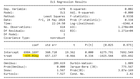
The regression output quantifies the data from the chart above. Without controlling for any additional variables, the treatment has a negative effect. Can we trust those results and conclude that the job training negatively impacted future earnings?
If that were the case, I wouldn't write an article about propensity score matching
