Combining Open Street Map and Landsat open data to verify areas of green zones

Today we would like to talk about the benefits of combining spatial data from various open data sources. For example, we will consider the following task: evaluating whether a particular property is located in a "green" area. Without further ado, let's get down to business!
P.S. Below, we consider a simple method of calculation based only on open data, covering most (I would like to believe all) of the cities. That's why below you will not see descriptions of machine learning approaches trained on such data, which is unlikely to be freely available.
Approach 1. The most accurate, but not for the lazy ones
Let's imagine that such an evaluation task occurred for a property in the city of Berlin at "Berlin, Neustädtische Kirchstraße 4–7". The task was given not by some full-time programmer, but, suppose, a person who can not program, but diligent and ready to learn something novel. After searching on the Internet, the "expert on assessing the greenness of the area" already downloaded QGIS and learned how to use the module Quick Map Services. The next steps may be obvious, but by far they are not easy: there is a need to figure out in what format spatial data are represented in geographic information systems (GIS) (vector and raster), then learn to create such objects and compare them with each other (to calculate the areas).

Despite the fact that along with the actions described above it is necessary to fill many other knowledge gaps (for example, what is a coordinate reference system and what they are), the most time-consuming process may be the creation of objects – vectorization. And while GIS operations will be easier and easier to do with knowledge and experience, vectorization is difficult to automate (it is almost always the case).
So, what can our specialist do? They can download Google Satellite data through the Quick Map Services module and manually label the data – draw the geometries of the objects themselves. In this case – parks and everything that looks like them. Then it will be able to put a buffer of 2,000 meters around (for example) the property to calculate its area. Then select those properties that lie in the same area and allocate them as green spaces, and calculate their area. The ratio "area of green areas in the neighborhood / area of the neighborhood" will be the value we are looking for.
An important clarification is to suggest that our specialist lives in Berlin and knows the investigated area well. Therefore, manually selected objects from the image can be considered as some combination of ground survey together with manual satellite image mapping.

Pros: Fairly accurate and objective estimation. The calculated ratio fully characterized the "greenness of the neighborhood". Our specialist will definitely get a bonus.
Cons: The proposed approach requires a lot of manual steps. Such work can't be done quickly (it took me 4 hours in total). Also we have to repeat a lot of the identical actions – such work can make our specialist work for a couple of weeks and go to a company where they will not make him/her count the green zones in such a way.
Approach 2. Cheap and cheerful
Surely we are talking about OpenStreetMap… Meanwhile our hero has realized that IT in general is much more interesting than real estate and started to learn Python programming language (of course). He/she got familiar with the osmnx module and geopandas library to process spatial data and shapely library to process geometries. With this trio, it is possible to perform a procedural evaluation of the greenness of an area. There is a need to perform the following steps:
- Create a polygon around the point (property) – the boundary of the area to analyze
- Query the OSM data that lie in this polygon (to query it, there is a need to figure out the tagging system that OSM has)
- Calculate areas at the area polygon and obtained geometries of parks and green areas according to OSM
Such an approach is much faster, since it doesn't require manual creation of polygons. Indeed, other people have already created these polygons for us – that's what makes the OSM great. However, OSM has disadvantages – the data may be inaccurate. Moreover, even if the polygons are rendered correctly by users, there is always a chance that we will just miscalculate the set of tags for a query and miss some important piece of data (Figure 2).

And there are quite a lot of these zones. Figure 2 shows only a small fraction. However, even this approach allows us to quickly and roughly, but still objectively assess the greenness of the area.
Pros: Fast and easy to evaluate. Despite inaccuracies, OSM data can be used in most cases
Cons: High estimation error if the source data is incorrect or if the set of tags to be queried is not detailed enough
Approach 3. Landsat images as a source of objective data
Oh, how much has been said and written about Landsat. And also about applications based on the calculated vegetation index NDVI. If you are interested, we suggest to check the following materials:
To make a long story short:
- Landsat is a satellite that flies over the Earth and takes images with a fairly high spatial resolution (from 15–30 in the optical spectrum to 100 meters in the far infrared spectrum)
- Normalized Difference Vegetation Index (NDVI) is a vegetation index that can be calculated from an image taken by Landsat. NDVI takes values from -1 to 1, where -1 means that in a given pixel there is nothing green at all (e.g. water), and 1 means that area in the pixel is very green – it is forest for example.
So, we can get a Landsat image (can be downloaded from here – search for "Landsat 8–9 OLI/TIRS C2 L2" product) for the selected area and calculate the NDVI. Then by varying the threshold we can segment the image into two classes: 0 – not green area and 1 – green area. We can vary the threshold as we want (Figure 3), but honestly, we don't know for sure which binarization threshold would work best. Moreover, this "optimal threshold" will be different for each new image obtained from Landsat: both for a new territory and for a different datetime index.

Pros: The approach provides up-to-date information about whether an area is green
Cons: Choosing the optimal threshold value is complicated – it is not clear which value to choose in order to separate vegetation from non-vegetation by threshold. There are sources, of course, where it is possible to find information about the proposed thresholds, for example, from 0.35 and above. But it is necessary to keep in mind that this optimal threshold value may change from image to image, from season to season, etc.
Approach 4. Areas by Landsat, thresholds by Openstreetmap
A reasonable solution to the threshold definition problem might be to use OSM data. Even though OSM data may have artifacts or missing some of the real-world objects, in general it gives a full picture of where objects (parks, squares, buildings) are located. So let's overlay the geometry mapping obtained from OSM and NDVI data, and then build a histogram (Figure 4).
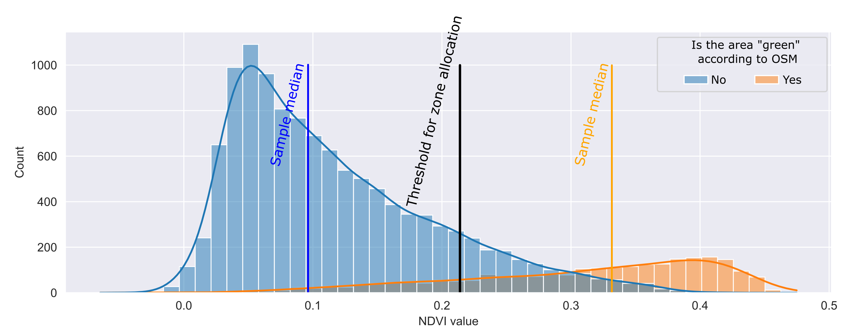
The black line in the figure shows a value that can be used as a threshold. Then it is possible to augment the OSM data with additional polygons obtained by automatic vectorization of the Landsat matrix. Thus, everything that is located to the right of the calculated threshold turns into "green zones". Due to this approach, the boundaries are extended (Figure 5).

Instead of a conclusion
There will be a picture…

As can be seen, the third approach with the adjustment of object boundaries using Landsat data turned out to be the closest to the benchmark (manual vectorization). The calculated values of the area also confirm that statement:
- (Benchmark) Manual vectorization: 25 %
- Calculation with OSM data: 17 %
- Calculation based on refined OSM and NDVI Landsat data: 28 %
As we can see, our estimate, although slightly overstated, is still much closer to actual values than the calculation according to OSM data. Moreover, our approach found green areas that we had not explored during manual vectorization – cemeteries in the north. If we exclude them from the analysis, the calculated areas will be much closer to the benchmark.
P.S. Based on this idea, we left the following artifacts:
- https://github.com/wiredhut/estaty – Python open-source library for processing spatial data and preparing MVP algorithms for real estate analysis. The library is pretty new, but we plan to develop and improve it
- http://api.greendex.wiredhut.com/ – service for calculating the "green" index and an internal tool (extension for google spreadsheets), so that we can conveniently work with the above algorithms both through API and through formulas in tables (for those who do not know how to code). This version uses a simplified calculation without using Landsat satellites
The story about combining OSM and Landsat data was told by Mikhail Sarafanov and Wiredhut team
