Data-Driven Dispatch

Introduction

In today's fast-paced world, the need for data-driven decisions in dispatch response systems is becoming essential. Dispatchers will perform a kind of triage when listening to calls, prioritising cases based on severity and time sensitivity among other factors. There is potential in optimising this process by leveraging the power of supervised learning models, to make more accurate predictions of case severity in tandem with a human dispatcher's assessment.

In this post, I'm going to run through one solution I developed to improve predictions of casualties and/or serious vehicular damage from car collisions in Chicago. Factors such as crash location, road conditions, speed limit, and time of occurrence were taken into account to answer a simple yes or no question – will this car crash require an ambulance or tow truck?

In a nutshell, this machine learning tool's primary objective is to classify collisions that will most likely require a callout (medical, tow, or both) based on other known factors. By leveraging this tool, responders would be able to efficiently allocate their resources across different parts of the city, based on various conditions such as weather and time of day.

For such a tool to be accurate and effective, a large data source would be needed to make predictions from the historical data – thankfully the city of Chicago already has such a resource (the Chicago Data Portal), so this data will be used as the test case.

Implementing these kinds of predictive models would certainly improve preparedness and response time efficiency when dealing with collisions on city streets. By gaining insights into the underlying patterns and trends within the collision data, we can work towards fostering safer road environments and optimising emergency services.

I go into the details of data cleaning, model building, fine tuning and evaluation below, before analysing the model's results and drawing conclusions. A link to the github folder for this project, which includes a jupyter notebook and a more comprehensive report on the project, can be found here.

---

Data Collection and Preparation

Initial Setup

I've listed the basic data analysis libraries used in the project below; standard libraries such as pandas and numpy were used throughout the project, along with matplotlib's pyplot and seaborn for visualisation. Additionally, I used the missingno library to identify gaps in the data – I find this library incredibly useful for visualising missing data in a dataset, and would recommend it for any data science project involving dataframes:

#generic data analysis 
import os
import pandas as pd
from datetime import date
import matplotlib.pyplot as plt
import numpy as np
import seaborn as sns
import missingno as msno

Functions from the machine learning module SciKit learn (sklearn) were imported to build the machine learning engine. these functions are shown here – I will describe the purpose of each of these functions in the Classification Model section later:

#Preprocessing
from sklearn.preprocessing import LabelEncoder
from sklearn.preprocessing import StandardScaler

# Models
from sklearn.neighbors import KNeighborsClassifier

# Reporting
from sklearn.model_selection import train_test_split
from sklearn.model_selection import RandomizedSearchCV

#metrics
from sklearn.metrics import accuracy_score
from sklearn.metrics import f1_score
from sklearn.metrics import precision_score
from sklearn.metrics import recall_score

The data for this project were all imported from the Chicago Data Portal, from two sources:

1. Traffic Crashes: Live dataset of vehicle collisions in the Chicago area. The features of this dataset are conditions recorded at the time of the collision, such as weather conditions, road alignment, latitude and longitude data, among other details.
2. Police Beats Boundaries: A static dataset indicating the boundaries of CPD beats; this dataset is used to supplement district information to the traffic crashes dataset. This can be joined to the original dataset to run analysis on districts with the most frequent collisions.

Data Cleaning

With both datasets imported, they can now be merged to add district data to the final analysis. This is done using the .merge() function in pandas – I used an inner join on both dataframes to capture all information in both, using the beat data in both as the join key (listed as beat_of_occurrence in the traffic crashes dataset, and BEAT_NUM in the police beats dataset):

#joining collision data to beat data - inner join
collisions = collision_raw.merge(beat_data, how='inner',
                                 left_on='beat_of_occurrence',
                                 right_on='BEAT_NUM'
                                 )

A quick look at the information provided from the .info() function shows a number of columns with sparse data. This can be visualized using the missingno matrix function:

#visualising missing data
#sorting values by report received date

collisions = collisions.sort_values(by='crash_date', ascending=True)

#plotting matrix of missing data
msno.matrix(collisions)
plt.show()

#info of sorted data
print(collisions.info())

This displays a matrix of missing data in all columns, as can be seen here:

By dropping columns with sparse data, a much cleaner dataset can be extracted; the columns to drop are defined in a list and then removed from the dataset using the .drop() function:

#defining unnecessary columns
drop_cols = ['location', 'crash_date_est_i','report_type', 'intersection_related_i',
       'hit_and_run_i', 'photos_taken_i', 'crash_date_est_i', 'injuries_unknown',
       'private_property_i', 'statements_taken_i', 'dooring_i', 'work_zone_i',
       'work_zone_type', 'workers_present_i','lane_cnt','the_geom','rd_no',
            'SECTOR','BEAT','BEAT_NUM']

#dropping columns
collisions=collisions.drop(columns=drop_cols)

#plotting matrix of missing data
msno.matrix(collisions)
plt.show()

#info of sorted data
print(collisions.info())

This leads to a much cleaner msno matrix:

Looking at the data for latitude and longitude, a small handful of rows had null values, and others mistakenly had zero values (most likely a reporting error):

These would cause errors in training the model, so I removed them:

#Some incorrect lat/long data - need to remove these rows
collisions = collisions[collisions['longitude']<-80]
collisions = collisions[collisions['latitude']>40]

With the data adequately cleaned, I was able to progress with developing the classification model.

---

Classification Model

Exploratory Data Analysis

Before proceeding with the Machine Learning model some exploratory data analysis (EDA) needs to be performed – each of the columns of the data frame are plotted on a histogram, with bins of 50 to show the distribution of the data. Histograms are useful in the EDA step for a number of reasons, namely that they give an overview of the data distribution, help to identify outliers, and ultimately assist in making decisions on feature engineering:

#plotting histograms of numerical values
collisions.hist(bins=50,figsize=(16,12))
plt.show()

A cursory look at the column histograms indicates that the latitude data is bimodal, while the longitude data is rightly skewed. This will need to be standardized so that it can be better applied for machine learning purposes.

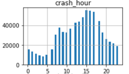
Additionally, it appears the crash hour column is cyclic in nature – this can be transformed using a trigonometric function (for example sine).

Scaling and Transformation

Scaling is a technique used in data preprocessing to standardise features so they have similar magnitudes. This is particularly important for machine learning models, since models are generally sensitive to the scale of input features. I've defined the StandardScaler() function to act as the scaler in this model – this scaling function transforms the data so that it has a mean of 0 and standard deviation of 1.

For data with a skewed or bimodal distribution, scaling can be done using logarithmic functions. Log functions make skewed data more symmetrical and reduce the tail on the data – this is useful when dealing with outlier values. I scaled the latitude and longitude data in this way; as the longitude data is all negative, the negative log was calculated and then scaled.

Python">#scaling latitude and longitude data
scaler = StandardScaler()

# Logarithmic transformation on longitude
collisions_ml['neg_log_longitude'] = scaler.fit_transform(np.log1p(-collisions_ml['longitude']).
                                                          values.reshape(-1,1))

# Normalisation on latitude
collisions_ml['norm_latitude'] = scaler.fit_transform(np.log1p(collisions['latitude']).
                                                      values.reshape(-1, 1))

This produces the desired effect, as can be seen below:

In comparison, cyclic data is usually scaled using trigonometric functions such as sine and cos. The crash hour data looks roughly cyclic based on earlier observations, so I applied a sine function to the data as below – since numpy's sin() function is in radians, I first converted the input to radians before calculating the sine of the input:

#transforming crash_hour 
#data is cyclic, can be encoded using trig transforms

#trig transformation - sin(crash_hr)
collisions_ml['sin_hr'] = np.sin(2*np.pi*collisions_ml['crash_hour']/24)

A histogram of the transformed data can be seen below:

Finally I removed the unscaled data from the model to avoid this interfering with model predictions:

#drop previous latitude/longitude columns
lat_long_drop_cols = ['longitude','latitude']
collisions_ml.drop(lat_long_drop_cols,axis=1,inplace=True)

#drop crash_hour column
collisions_ml.drop('crash_hour',axis=1,inplace=True)

Data Encoding

Another important step in data preprocessing is data encoding – this is where non-numerical data (for example categories) are represented in numerical format, to make it compatible with machine learning algorithms. For categorical data in this model, I used a method called label encoding – each category in a column is given a numerical value before it's inputted to the model. A diagram of this process is shown below:

I encoded the columns in the dataset, first segmenting out the columns I wanted to keep from the original dataset and making a copy of the dataframe (collisions_ml). I then defined the categorical columns in a list, and used the LabelEncoder() function from sklearn to fit and transform the categorical columns:

#segmenting columns into lists
ml_cols = ['posted_speed_limit','traffic_control_device', 'device_condition', 'weather_condition',
          'lighting_condition', 'first_crash_type', 'trafficway_type','alignment', 
           'roadway_surface_cond', 'road_defect', 'crash_type','damage','prim_contributory_cause',
          'sec_contributory_cause','street_direction','num_units', 'DISTRICT',
          'crash_hour','crash_day_of_week','latitude', 'longitude']
cat_cols = ['traffic_control_device', 'device_condition', 'weather_condition', 'DISTRICT',
           'lighting_condition', 'first_crash_type', 'trafficway_type','alignment',
           'roadway_surface_cond', 'road_defect', 'crash_type','damage','prim_contributory_cause',
           'sec_contributory_cause','street_direction','num_units']

#making a copy of the dataset
collisions_ml = collisions[ml_cols].copy()

#encoding categorical values
label_encoder = LabelEncoder()
for col in collisions_ml[cat_cols].columns:
    collisions_ml[col] = label_encoder.fit_transform(collisions_ml[col])

With the data now sufficiently preprocessed, the data can now be split into train and test data, and a classification model can be fitted to the data.

Splitting the Train & Test Data

It's important to separate data into a training and test sets when building a machine learning model; the training set is a fraction of the initial data which is used to train the model on the right responses, whereas the test set is used to evaluate model performance. Keeping these separate is necessary to reduce the risk of overfitting and model bias.

I separated out the crash_type column using the drop() function (the remaining features will be used as the variables to predict crash_type), and defined crash_type as the y result to be predicted using the model. The train_test_split function from sklearn was used to take 20% of the initial dataset as training data, with the rest to be used for model testing.

#Create test set
#setting X and y values

X = collisions_ml.drop('crash_type', axis=1)
y = collisions_ml['crash_type']
X_train, X_test, y_train, y_test = train_test_split(X, y, test_size=0.2, random_state=42)

K-Nearest Neighbors Classification

For this project, a K-Nearest Neighbors (KNN) classification model is used to predict results from the features. KNN models work by checking the value of the K nearest known values around an unknown data point, then classifying the data point based on the values of those "neighbor" points. It's a non-parametric classifier, meaning it doesn't make any assumptions about the underlying data distribution; however it is computationally expensive, and can be sensitive to outliers in the data.

I instantiated the KNN classifier with an initial n_neighbors equal to 3, using Euclidean metrics, before fitting the model to the training data:

#Classifier - K Nearest Neighbours
#instantiate KNN Classifier
KNNClassifier = KNeighborsClassifier(n_neighbors=3, metric = 'euclidean')

KNNClassifier.fit(X_train,y_train)

Once the model was fitted to the training data, I made predictions on the test data as below:

#Predictions
#predict on training set
y_train_pred = KNNClassifier.predict(X_train)

#predict on test data
y_test_pred = KNNClassifier.predict(X_test)

Evaluation

Evaluation of a machine learning model is typically done using four metrics; accuracy, precision, recall, and F1 score. The differences between these metrics are very subtle, but in plain English these terms can be defined as follows:

1. Accuracy: the percentage of true positive predictions out of all model predictions. Typically the accuracy of both the train and test data should be measured to evaluate model fit.
2. Precision: the percentage of true positive predictions out of all positive model predictions.
3. Recall: the percentage of true positive predictions out of all positive cases in the dataset.
4. F1 Score: An overall metric of the model's ability to identify positive instances in the data, combining the precision and recall scores.

I computed the metrics of the KNN model using the below code snippet – I also calculated the difference between the model's accuracy on the train and test set, to assess fit:

#Evaluate model
# Calculate the accuracy of the model

#calculating accuracy of model on training data
train_accuracy = accuracy_score(y_train, y_train_pred)

#calculating accuracy of model on test data
test_accuracy = accuracy_score(y_test, y_test_pred)

#computing f1 score,precision,recall
f1 = f1_score(y_test, y_test_pred)
precision = precision_score(y_test,y_test_pred)
recall = recall_score(y_test,y_test_pred)

#comparing performances
print("Training Accuracy:", train_accuracy)
print("Test Accuracy:", test_accuracy)
print("Train-Test Accuracy Difference:", train_accuracy-test_accuracy)

#print precision score
print("Precision Score:", precision)

#print recall score
print("Recall Score:", recall)

#print f1 score
print("F1 Score:", f1)

The initial metrics of the KNN model are given below:

The model scored well on test accuracy (79.6%), precision (82.1%), recall (91.1%), and F1 score (86.3%) – however the test accuracy was much higher than the train accuracy at 93.1%, a 13.5% difference. This indicates the model is overfitting the data, which means it would struggle to accurately make predictions on unseen data. Therefore the model needs to be adjusted for a better fit – this can be done using a process called hyperparameter tuning.

Hyperparameter Tuning

Hyperparameter tuning is the process of selecting the best set of hyperparameters for a machine learning model. I fine-tuned the model using k-fold cross-validation – this is a resampling technique where the data is split into k subsets (or folds), then each fold in turn is used as the validation set while the remaining data is used as the training set. This method is effective at reducing the risk of bias being introduced to the model by a particular choice of training/test set.

The hyperparameters for the KNN model are number of neighbors (_nneighbors) and the distance metric. There are a number of different ways to measure distance in a KNN classifier, but here I focused on two options:

1. Euclidean: This can be thought of as the straight-line distance between two points – it's the most commonly used distance metric.
2. Manhattan: Also called "city block" distance, this is the sum of absolute differences between the coordinates of 2 points. If you imagine standing at the corner of a city building and trying to get to the opposite corner – you wouldn't cross through the building to get to the other side, but instead go up one block, then across one block.

Note that I could have also fine-tuned the weight parameter (which determines whether all neighbors vote equally or if the closer neighbors are given more importance), but I decided to keep the voting weight uniform.

I defined a parameter grid with n_neighbors of 3, 7, and 10, as well as metrics of Euclidean or Manhattan. I then instantiated a RandomizedSearchCV algorithm, passing in the KNN classifier as the estimator, along with the parameter grid. I set the algorithm to split the data into 5 folds by setting the cv parameter to 5; this was then fit to the training set. A snippet of the code for this can be seen below:

#Fine tuning (RandomisedSearchCV)
# Define parameter grid
param_grid = {
    'n_neighbors': [3, 7, 10],
    'metric': ['euclidean','manhattan']
}

# instantiate RandomizedSearchCV
random_search = RandomizedSearchCV(estimator=KNeighborsClassifier(), param_distributions=param_grid, cv=5)

# fit to training data
random_search.fit(X_train, y_train)

# Retrieve best model and performance
best_classifier = random_search.best_estimator_
best_accuracy = random_search.best_score_

print("Best Accuracy:", best_accuracy)
print("Best Model:", best_classifier)

The best accuracy and classifier were retrieved from the algorithm, indicating the classifier performs best with n_neighbors set to 10 while using the Manhattan distance metric, and that this would lead to an accuracy score of 74.0%:

as such these parameters were inputted to the classifier, and the model was retrained:

#Classifier - K Nearest Neighbours
#instantiate KNN Classifier
KNNClassifier = KNeighborsClassifier(n_neighbors=10, metric = 'manhattan')

KNNClassifier.fit(X_train,y_train)

Performance metrics were again extracted from the classifier, in the same manner as before – a screengrab of the metrics for this iteration can be seen below:

Cross-validation led to slightly poorer results for all metrics; test accuracy dropped by 2.6%, precision by 1.5%, recall by 0.5%, and F1 score by 1%. however the training-test accuracy difference dropped to 3.8%, where it was initially 13.5%. This indicates the model is no longer overfitting the data, and is therefore more suitable for predicting unseen data.

Conclusion

In summary, the KNN classifier performed well in predicting whether a collision would require a tow or ambulance. Initial metrics from the model's first iteration were impressive, however the disparity between test and training accuracy indicated overfitting. Hyperparameter tuning allowed for the model to be optimised, which significantly reduced the gap in accuracies between the two datasets. While performance metrics did take a small hit during this process, the benefit of a model with better fit outweighs these concerns.

References

1. Levy, J. (n.d.). Traffic Crashes – Crashes [Dataset]. Retrieved from Chicago Data Portal. Available at: https://data.cityofchicago.org/Transportation/Traffic-Crashes-Crashes/85ca-t3if (Accessed: 14th May 2023).
2. Chicago Police Department. (n.d.). Boundaries – Police Beats (current) [Data set]. Retrieved from Chicago Data Portal. Available at: https://data.cityofchicago.org/Public-Safety/Boundaries-Police-Beats-current-/aerh-rz74 (Accessed: 14th May 2023).
3. Zach M. (2022). "How to Perform Label Encoding in Python (With Example)." [Online]. Available at: https://www.statology.org/label-encoding-in-python/ (Accessed: July 19th, 2023).

Tags: Classification Data Science Data Visualization Machine Learning Python

Comment