Deep Learning Illustrated, Part 4: Recurrent Neural Networks
Welcome to Part 4 of our illustrated Deep Learning journey! Today, we're diving into Recurrent Neural Networks. We'll be talking about concepts that will feel familiar, such as inputs, outputs, and activation functions, but with a twist. And if this is your first stop on this journey, definitely read the previous articles, particularly Parts 1 and 2, before this one.
Recurrent Neural Networks (RNN) are unique models explicitly designed to handle sequence-based problems, where the next position relies on the previous state.
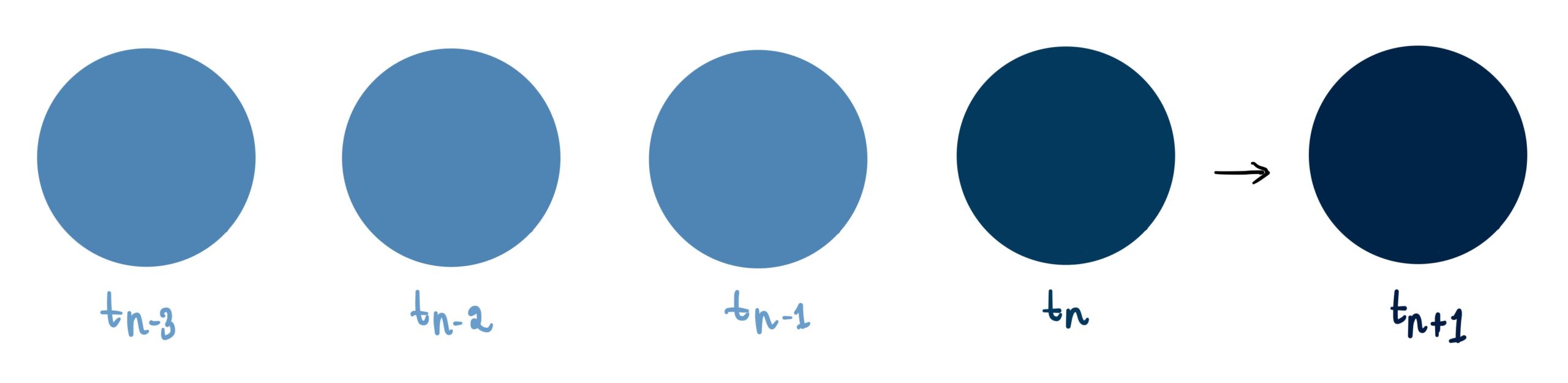
Let's unpack what a sequence-based problem is with a simple example from this MIT course. Picture a ball at a specific point in time, tn.

If we're asked to predict the ball's direction, without further information, it's a guessing game – it could be moving in any direction.

But what if we were provided with data about the ball's previous positions?

Now we can confidently predict that the ball will continue moving to the right.
This prediction scenario is what we call a sequential problem – where the answer is strongly influenced by prior data. These sequential problems are everywhere, from forecasting tomorrow's temperature based on past temperature data to a range of language models including sentiment analysis, named entity recognition, machine translation, and speech recognition. Today, we'll tackle sentiment detection, a straightforward example of a sequence-based problem.
In sentiment detection, we take a piece of text and determine whether it conveys a positive or negative sentiment. Today we're going to build an RNN that takes a movie review as an input and predicts whether it is positive or not. So, given this movie review…

…we want our neural network to predict that this has a positive sentiment.
This may sound like a straightforward classification problem, but standard neural networks face two major challenges here.
First, we're dealing with a variable input length. A standard neural network struggles to process inputs of differing lengths. For example, if we train our neural network with a three-word movie review, our input size will be fixed at three. But what if we want to input a longer review?

It would be stumped and unable to process the above review with twelve inputs. Unlike previous articles where we had a set number of inputs (the ice cream revenue model had two inputs – temperature and day of the week), in this case, the model needs to be flexible and adapt to however many words are thrown its way.
Second, we have sequential inputs. A typical neural network doesn't fully understand the directionality of the inputs, which is critical here. Two sentences might contain the exact same words, but in a different order, they can convey completely opposite meanings.

Given these challenges, we need a method to process a dynamic number of inputs sequentially. Here's where the RNNs shine.
The way we approach this problem is to first process the first word of the review, "that":

Then use this information to process the second word, "was":

And finally, use all of the above information to process the last word, "phenomenal", and provide a prediction for the sentiment of the review:

Before we start building our neural network, we need to discuss our inputs. Inputs to a neural network must be numerical. However, our inputs here are words, so we need to convert these words into numbers. There are several ways to do this, but for today, we'll use a basic method.
Stay tuned for an upcoming article where we'll explore more sophisticated methods to address this challenge.
For now, let's imagine we have a large dictionary of 10,000 words. We'll (naively) assume that any words appearing in the reviews can be found within this 10,000-word dictionary. Each word is mapped to a corresponding number.

To convert the word "that" to a bunch of numbers, we need to identify the number "that" is mapped to…

…and then represent it as matrix of 10,000 0's except the 8600th element which is a 1:

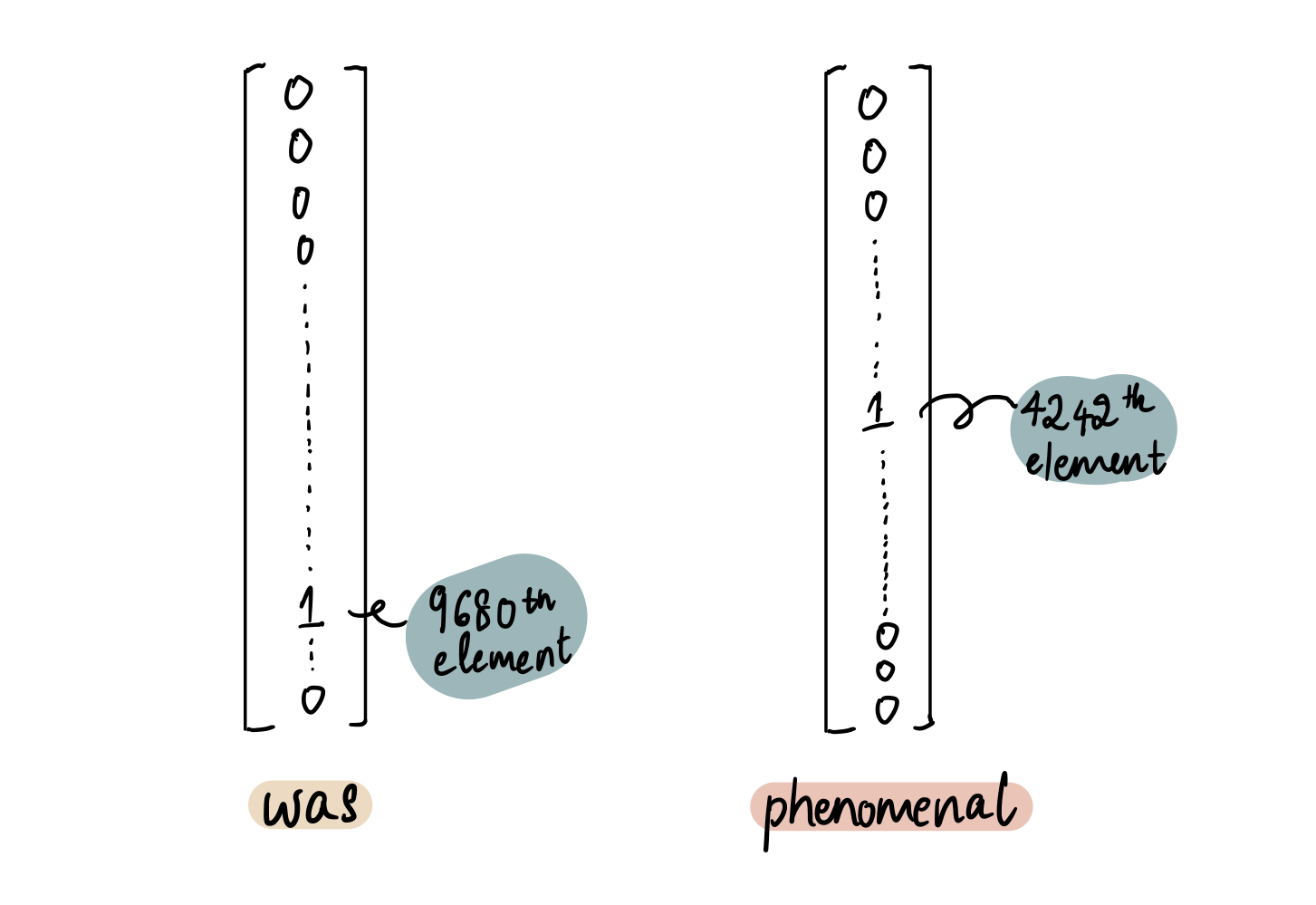
Similarly, the numerical representations for the next two words, "was" (9680th word in the dictionary) and "phenomenal" (4242th word in the dictionary), will be:
And that's how we take a word and convert it into a neural network-friendly input.
Let's now turn our attention to the design of the neural network. For the sake of simplicity, let's assume our network has 10,000 inputs (= 1 word), a single hidden layer composed of one neuron, and one output neuron.

And of course, if this is a fully trained neural network, then each input will have associated weights and the neurons will have bias terms.

In this network, the input weight are labeled as wᵢ, where i denotes the input. The bias term in the hidden layer neuron is bₕ. The weight connecting the hidden layer to the output neuron is wₕᵧ. Finally, the bias in the output neuron is represented by bᵧ, as y indicates our output.
We will use the hyperbolic tangent function (tanh) as the activation function for the hidden neuron.

And as a refresher from the first article, tanh takes an input and produces an output within the range of -1 to 1. Large positive inputs tend towards 1, while large negative inputs approach -1.

To determine the sentiment of the text, we could use the sigmoid activation function in the output neuron. This function takes the output from the hidden layer and outputs a value between 0 and 1, representing the probability of positive sentiment. A prediction closer to 1 indicates a positive review, while a prediction closer to 0 suggests that it is not likely to be positive.

While this method works for now, there is a more sophisticated approach that could yield better results! If you stick around to very end of the article, you'll see a new and powerful and ubiquitous activation function – Softmax Activation – that tackles this problem better.
With these activation functions, our neural network looks like this:

This neural network takes a text input and predicts the probability of it having a positive sentiment. In the above example, the network processes the input "that" and predicts its likelihood of being positive. Admittedly, the word "that" on its own doesn't provide much hint as to the sentiment. Now, we need to figure out how to incorporate the next word into the network. This is when the recurrent aspect of recurrent neural networks comes into play, leading to a modification in the basic structure.
We input the second word of the review, "was" by creating an exact copy of the above neural network. However, instead of using "that" as the input, we use "was":

Remember, we also want to use the information from the previous word, "this" in this neural network. Therefore, we take the output from the hidden layer of the previous neural network and pass it into the hidden layer of the current network:

This is a crucial step, so let's break it down slowly.
From the [first article](https://towardsdatascience.com/neural-networks-illustrated-part-1-how-does-a-neural-network-work-c3f92ce3b462), we learned that each neuron's processing consists of two steps: summation and activation function (please read the first article if you're unsure of what these terms mean). Let's see what this looks like in our first neural network.

In the hidden layer neuron of the first neural network, the first step is summation:

Here, we multiply each of the inputs by their corresponding weights and add the bias term to the sum of all the products:

To simplify this equation, let's represent it this way where wₓ represents the input weights and x represents the input:

Next, in step 2, we pass this summation through the activation function, tanh:


This produces the output h₁ from the hidden layer of the first neural network. From here, we have two options – pass h1 to the output neuron or pass it to the hidden layer of the next neural network.
(option 1) If we want the sentiment prediction for just "that", then we can take h₁ and pass it to the output neuron:

For the output neuron, we perform the summation step…


…and then apply the sigmoid function to this sum…

…which gives us our predicted positive sentiment value:

So this _y₁hat gives us the predicted probability that "that" has a positive sentiment.
(option 2) But that's not what we want. So instead of passing h₁ to the output neuron, we pass this information to the next neural network like so:

Similar to other parts of the neural network where we have input weights, we also have an input weight, wₕₕ, for the input from one hidden layer to another. The hidden layer incorporates h₁ by adding the product of h₁ and wₕₕ to the summation step in the hidden neuron. Therefore, the updated summation step in the hidden neuron of the second neural network neuron will be:


Key thing to note – all the bias and weight terms throughout the network remain unchanged since they are simply copies from the previous network.
This sum is then passed through the tanh function…

…producing h₂, the output from the hidden layer in the second neural network:

From here, again, we can obtain a sentiment prediction by passing h₂ through the output neuron:


Here, _y₂hat yields the predicted probability that "that was" has a positive sentiment.
But we know that's not the end of the review. So, we will replicate this process where we clone this network once again but with the input "phenomenal" and pass the previous hidden layer output to the current hidden layer.

We process the hidden layer neuron…

…to an output, h₃:

Since this is the last word in the review and consequently the final input, we pass this data to the outer neuron…

…to give us a final prediction of the sentiment:

And this _y₃hat is the sentiment of the movie review we want and is how we achieve what we drew out in the beginning!
Formal Representation
If we flesh out the above diagram with details, then we'll get something like this:

Each stage of the process involves an input, x, that travels through the hidden layer to generate an output, h. This output then either moves into the hidden layer of the next neural network or it results in a sentiment prediction, depicted as _yhat. Each stage incorporates weight and bias terms (bias is not shown in the diagram). A key point to underscore is that we're consolidating all the hidden layers into a singular compact box. While our model only contains one layer with a single neuron in the hidden layer, more complex models could include multiple hidden layers with numerous neurons, all of which are condensed into this box, called the hidden state. This hidden state encapsulates the abstract concept of the hidden layer.
Essentially, this is a simplified version of this neural network:

It's also worth noting that we can represent all of this in this streamlined diagram for simplicity:

The essence of this process is the recurrent feeding of the output from the hidden layer back into itself, which is why it's referred to as a recurrent neural network. This is often how neural networks are represented in textbooks.
From a mathematical standpoint, we can boil this down to two fundamental equations:

The first equation encapsulates the full linear transformation that takes place within the hidden state. In our case, this transformation is the tanh activation function within the individual neuron. The second equation denotes the transformation happening in the output layer, which is the sigmoid activation function in our example.

What type of problems does an RNN solve?
Many-to-One
We just discussed this scenario where multiple inputs (in our case, all the words in a review) are fed into an RNN. The RNN then generates a single output, representing the sentiment of the review. While it's possible to have an output at every step, our primary interest lies in the final output, as it encapsulates the sentiment of the entire review.

Another example is text completion. Given a string of words, we want the RNN to predict the next word.

One-To-Many

A classic example of a one-to-many problem is image captioning. Here, the single input is an image and the output is a caption consisting of multiple words.
Many-to-Many

This type of RNN is used for tasks like machine translation, for instance, translating an English sentence into Hindi.
Drawbacks
Now that we've unpacked how an RNN works, it's worth addressing why they're not as widely used (plot twist!). Despite their potential, RNNs face significant challenges during training, particularly due to something called the Vanishing Gradient Problem. This problem tends to intensify as we unroll the RNN further, which in turn, complicates the training process.
In an ideal world, we want the RNN to take into account both the current step input and the ones from the previous steps equally:

However, it actually looks something like this:

Each step slightly forgets the previous one, leading to a short-term memory problem known as the vanishing gradient problem. As the RNN processes more steps, it tends to struggle with retaining information from previous ones.
With only three inputs, this issue isn't too pronounced. But what if we have six inputs?

We see that the information from the first two steps is almost absent in the final step, which is a significant issue.
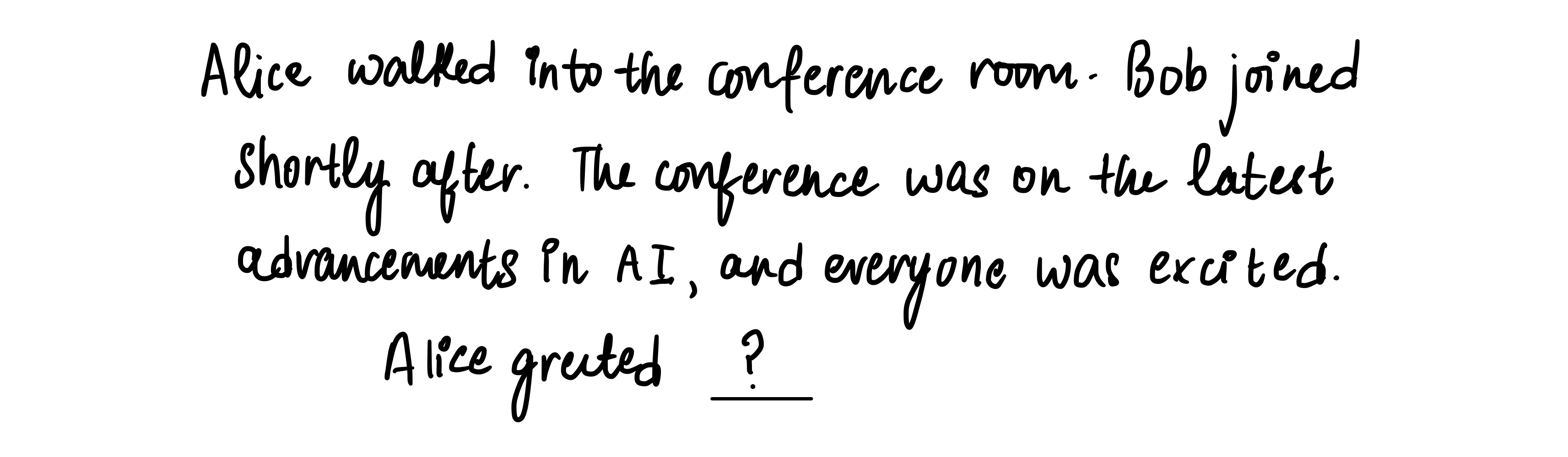
Here's an example to illustrate this point using a text completion task. Given this sentence to complete, an RNN might be successful.
However, if more words are added in between, the RNN might struggle to predict the next word accurately. This is because the RNN could potentially forget the context provided by the initial words due to the increased distance between them and the word to be predicted.
This highlights the fact that while RNNs sound great in theory, they often fall short in practice. To address the short-term memory issues, we use specialized types of RNNs known as Long Short-Term Memory (LSTM) networks, which is covered in Part 5 of the series!
Deep Learning Illustrated, Part 5: Long Short-Term Memory (LSTM)
Bonus: Softmax Activation Function
We spoke earlier about an alternate, much better way of tackling our sentiment prediction. Let's take a few steps back to the drawing board and go back to when we were deciding on the activation function for our output neuron.

But our focus this time is a bit different. Let's zoom in on a basic neural network, setting aside the recurrent aspects. Our goal now? To predict the sentiment of a single input word, not the entire movie review.
Previously, our prediction model aimed to output the probability of a input being positive. We accomplished this using the sigmoid activation function in the output neuron, which churns out probability values for the likeliness of a positive sentiment. For instance, if we input the word "terrible", our model would ideally output a low value, indicating a low likelihood of positivity.

However, thinking about it, this isn't that great of an output. A low probability of a positive sentiment doesn't necessarily imply negativity – it could also mean that the input was neutral. So, how do we improve this?
Consider this: What if we want to know whether the movie review was positive, neutral, or negative?
So instead of just one output neuron that spits out the probability prediction that the input is positive, we could use three output neurons. Each one would predict the likelihood of the review being positive, neutral, and negative, respectively.

Just as we used the sigmoid function for a single-output neuron network to output probability, we could apply the same principle to each of these neurons in our current network and use a sigmoid function in all of them.

And each neuron will output its respective probability value:

However, there's a problem: the probabilities don't sum up correctly (0.1 + 0.2 + 0.85 != 1) so this isn't such a great workaround. Simply sticking a sigmoid function for all the output neurons doesn't fix the problem. We need to find a way to normalize these probabilities across the three outputs.
Here's where we introduce a powerful activation function to our arsenal – the softmax activation. By using the softmax activation function, our neural network takes on a new form:

While it may seem daunting at first, the softmax function is actually quite straightforward. It simply takes the output values (_yhat) from our output neurons and normalizes them.
However, it's crucial to note that for these three output neurons, we won't use any activation function; the outputs (_yhats) will be the result we obtain directly after the summation step.
If you need a refresher of what the summation step and activation step in the neuron entail, this article in the series goes over the inner workings of a neuron in detail!
We normalize these _yhat outputs through the use of the softmax formula. This formula provides the prediction for the probability of a positive sentiment:

Similarly, we can also obtain the prediction probabilities of negative and neutral outcomes:


Let's see this in action. For instance, if "terrible" is our input, these will be the resulting _yhat values:

We can then take these values and plug them into the softmax formula to calculate the prediction probability that the word "terrible" has a positive connotation.

This means that by using the combined outputs from the sentiment neuron, the probability that "terrible" carries a positive sentiment is 0.05.
If we want to calculate the probability of the input being neutral, we would use a similar formula, only changing the numerator. Therefore, the likelihood of the word "terrible" being neutral is:

And probability prediction that "terrible" is negative is:

And voila! Now the probabilities add up to 1, making our model more explainable and logical.
So, when we ask the neural network – "What's the probability that "terrible" has a negative sentiment attached to it?", we get pretty a straightforward answer. It confidently states that there is an 85% probability that "terrible" has a negative sentiment. And that's the beauty of the softmax activation function!
That's a wrap for today! We've tackled two biggies – Recurrent Neural Networks and the Softmax Activation Function. These are the building blocks for many advanced concepts we'll dive into later. So, take your time, let it sink in, and as always feel free to connect with me on LinkedIn or shoot me an email at [email protected] if you have any questions/comments!
NOTE: All illustrations are by the author unless specified otherwise
