Estimating Total Experimentation Impact

Introduction

Data-driven organizations often run hundreds or thousands of experiments at any given time, but what is the net impact of all of these experiments? A naive approach is to sum the difference-in-means across all experiments that resulted in a significant and positive treatment effect and that were rolled out into production. This estimate, however, can be extremely biased, even if we assume there are no correlations between individual experiments. We will run a simulation of 10,000 experiments and show that this naive approach overestimates the actual impact delivered by 45%!

We review a theoretical bias correction formula, due to Lee and Shen [1]. This approach, however, suffers from two defects: first, though it is theoretically unbiased, we show that its corresponding plug-in estimator nonetheless suffers from significant bias for similar reasons as the original problem. Second, it does not attribute impact to individual level experiments.

In this post, we explore two sources of bias:

• False-discovery bias – the estimate is inflated due to false positives;
• Selection bias – the estimate is inflated due to a bias introduced by the decision criterion: underestimates of the treatment effect are censored (false negatives), whereas overestimates are rewarded.

To address false discovery, we will construct a probability that a given result is actually non-zero. This probability is constructed by comparing the p-value density to the referred residual density from the true nulls.

To address selection bias, we will compute a posterior distribution for each experimental result, using the empirical distribution, corrected for false discovery, as our prior.

This process yields an accurate estimate of the average experimental impact across our simulated series of experiments, reducing the original 45% error using the empirical measurements alone to a 0.4% error.

The Effect Distribution

So we've ran a bunch of experiments and want to quantify our total experimental impact delivered. To do this, we need to consider the effect distribution, or the distribution of treatment effects. To conceptualize this, imagine running many many experiments. Each experiment will have a true value of its effect θᵢ, which we may regard as a random variable drawn from some true effect distribution p. Each experiment then estimates θᵢ through Xᵢ (which we may regard as the average difference-in-means). We thus obtain the following model for our observations:

Here, σᵢ² ~ 1/nₛ, where nₛ is the sample size. We will consider the true effect distribution to be a mixture of three subpopulations: true nulls, positives, and negatives. To describe the effect distribution, we consider three parameters:

• λ = P(θ != 0) (effectiveness): the fraction of experiments with a nonzero effect,
• κ = P(θ > 0 | θ != 0) (asymmetry): the fraction of experiments with positive effect, out of those that have a nonzero effect,
• ρ = P(θ > δ | θ > 0) (advantage): the fraction of experiments with a practically significant effect (i.e., whose effect size is greater than δ), out of those that have a positive (significant) effect.

These parameters are illustrated in the figure below.

For newer products, it may be easy to come up with feature ideas that result in a significant effect, so that λ would be high. For mature products, however, it may be the case that it is very rare for an experiment to lead to a significant change, and λ would be low.

Similarly, a given team might be very good at proposing product-change ideas that actually result in a positive effect, so that κ > 1/2, but another team might propose a bunch of bad ideas that result in performance loss, so that that the effects tend to be negative, so that κ < 1/2.

Theoretical Bias Estimator

Consider the random set A consisting of the positive significant results from a series of experiments, with decision criterion _Xi > c. Define the total true and estimated effects as

The total expected bias can be described as b = E[Sₐ— Tₐ]. If Xᵢ ~ N(θᵢ, σᵢ), Lee and Shen [1] show that the total expected bias is given by:

where ϕ is the density of the standard normal distribution. The details of this are further reviewed in [2]. There are two main drawbacks to this formula:

1. It relies on the true effects θᵢ. To actually use it, we must therefore replace the true effects with the observed effects, the so-called plug-in estimator. In our simulation, we show that the plug-in estimator can lead to a significantly biased estimate. (We will also show how to correct for this by taking into account false-discovery.)
2. The summation is over all experiments, not limited to those with a positive significant result. So even correcting for the first problem, it does not provide an estimate of impact at the individual experiment level, the so-called attribution problem.

Simulating an Experimentation Platform

A Few Assumptions

Let's start by making a few assumptions about the set of experiments we are analyzing:

• each experiment measures the difference-in-means for the same top-line metric (e.g., DAUs, time spent, revenue);
• each experiment was run using the same significance level α and power β for effect size δ (which is the minimum effect that would be practically significant);
• each experiment therefore has the same sample size nₛ and rejection criterion Xᵢ > c.

For purposes of calculation, we will use α = 0.05, β = 0.8 for effect size δ = 0.1, which yield c = 0.07 and nₛ = 785. Note: we regard α as a two-sided significance. The actual significance for the positive test is α/2.

Simulation in Python

We next construct a simulated experimentation platform in Python, as shown below.

class PlatformSim:
    def __init__(self, alpha=0.05, beta=0.80, delta=0.1):
        self.alpha, self.beta, self.delta = alpha, beta, delta
        self.z_crit = stats.norm.isf(self.alpha/2)
        self.n_s = int(np.ceil(delta**(-2) * (stats.norm.isf(alpha/2) - stats.norm.isf(beta))**2))
        self.theta_crit = self.z_crit / np.sqrt(self.n_s)

    def run(self, n, lambda_=0.2, kappa=0.5, rho=0.2, shape=3):
        self.n_null = int(n * (1 - lambda_))
        self.n_pos = int(n * lambda_ * kappa)
        self.n_neg = n - self.n_null - self.n_pos 
        # compute thetas
        thetas_null = np.zeros(self.n_null)
        scale = self.delta / scipy.stats.gamma.isf(rho, shape)
        thetas_pos = +np.random.gamma(shape, scale=scale, size=self.n_pos)
        thetas_neg = -np.random.gamma(shape, scale=scale, size=self.n_neg)
        self.thetas = np.concatenate((thetas_null, thetas_pos, thetas_neg))
        # for each theta, simulate result of an experiment        
        np.random.shuffle(self.thetas)
        self.x_values, self.z_values, self.p_values = self.simulate_results(self.thetas)
        self.results = (self.z_values > self.z_crit).astype(int)

    def simulate_results(self, thetas):
        X = np.random.normal(loc=thetas, size=(self.n_s, len(thetas)))
        self.X = X
        x_values = X.mean(axis=0)
        z_values = x_values * np.sqrt(self.n_s)
        p_values = 2 * stats.norm.sf(np.abs(z_values))
        return x_values, z_values, p_values

We first assign (1-λ) of the experiments to have a true null effect.

For the remainder of experiments, we use a gamma distribution, ensuring that the survival function at δ is ρ.

With the PlatformSim class, we can run a simulation with a few lines of code. We put the results into a dataframe df, and create a separate dataframe dfs for positive results. Note: this can be easily modified to model different distributions for the positive / negative wings. For the purpose of our simulation, however, we used a gamma random variable.

P = PlatformSim(alpha=0.05, beta=0.8, delta=0.1)
P.run(10000, lambda_= 0.2, kappa=0.5, rho=0.3, null_type=null_type, pos_type=pos_type, shape=3)
df = DataFrame({'theta': P.thetas, 'x': P.x_values, 'z': P.z_values, 'p': P.p_values, 'result': P.results})
df.sort_values('p', inplace=True, ignore_index=True)
dfs = df[df.result==1]
effect = dfs.theta.mean()
print(f"Average Effect (Actual): {round(effect, 6)}")  
print(f"Average Effect (Observed): {round(dfs.x.mean(), 6)}     REL: {100*round(dfs.x.mean() / effect - 1, 2)}%")  
print(f"False Discovery Rate: {round(100*len(dfs[dfs.theta <= 0]) / len(dfs), 2)}%") 
sig_i = 1 / np.sqrt(P.n_s)
imp_b = (dfs.x.sum() - sig_i * scipy.stats.norm.pdf((P.theta_crit - df.x) / sig_i).sum()) / len(dfs)
imp_0 = (dfs.x.sum() - sig_i * scipy.stats.norm.pdf((P.theta_crit - df.theta) / sig_i).sum()) / len(dfs)
print(f"Bias-Corrected True      Estimate: {round(imp_0, 6)}     REL: {round(100* imp_0 / dfs.theta.mean() - 100, 2)}%")
print(f"Bias-Corrected Empirical Estimate: {round(imp_b, 6)}     REL: {round(100* imp_b / dfs.theta.mean() - 100, 2)}%")
# Output ~
# Average Effect (Actual): 0.079171
# Average Effect (Observed):  0.113245    REL: 43.0%
# False Discovery Rate:  27.04%
# Bias-Corrected True      Estimate:  0.079023     REL: -0.19%
# Bias-Corrected Empirical Estimate:  0.062471     REL: -21.09%

Using our simulation, we can easily measure both the observed average treatment effect as well as the actual treatment effect, for experiments that had a significant and positive effect. In this simulation, the true average effect is 0.0792, whereas our measured effect is 0.1132, a +43% error! We also observe a false-discovery rate of 27%.

We also observe that the theoretical bias-correction formula works perfectly when using the true _θᵢ_s, with a 0.19% error, but fails when swapped for the plug-in estimator, which produces a 21% error. The theoretical estimator overcorrects for bias. This is due to the large number of true nulls and the fact that the bias formula picks up observations randomly scattered to the right, but not those scattered to the left, as the estimator value peaks for observed values near the decision boundary.

We can plot a histogram of the effect distribution. Below is a histogram of the true effects, with the positive test results highlighted in orange.

We notice there are a large number of false positives, much more than our α/2 = 2.5% positive significance level. The fraction of false positives to overall positives is known as the false discovery rate, and we will discuss how to estimate it and adjust for it momentarily.

Now, when conducting a series of experiments, one would not have access to this true distribution of treatment effects, but instead only to the distribution of observed treatment effects, which is plotted below. Here, we highlight those experiments in which the true effect actually was positive in orange. This view gives us insight into the second type of bias we must address: selection bias.

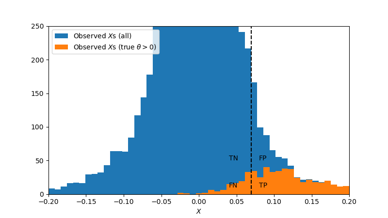
To understand selection bias, consider that the false negatives have true effects to the right of the vertical dashed line. For every experiment scattered to the left, one will be scattered to the right. So the false negatives may be regarded as a reflection of true positives that are overestimates. The selection process itself therefore creates a bias: only if the observed effect is greater than c do we consider the result to be statistically significant. We are therefore selecting the observations that randomly have a higher effect than their true effect, and ignoring the observations that have a lower effect. All of the false negatives highlighted in the above figure "balance out" with a true positives whose measured effect is inflated.

False Discovery

In this section, we discuss some theoretical relationships between λ, κ, power, and the false-discovery rate. We will use these in our simulation later in this note.

Estimating λ and κ

In order to estimate the false-discovery rate using the observational data that would be available in practice, we need to first estimate the population parameters λ and κ.

To estimate λ, we consider the fraction f of experiments that led to statistically significant results. These consist of true positives and false positives . Of the (1-λ) experiments with no effect, we expect α (1 – λ) to produce false positives. Of the λ experiments with an actual effect, we expect βₐ λ to produce true positives, where βₐ is the average power over this set of experiments. The expected fraction of significant results is therefore given by

which may be rearranged to produce the estimate

where βₐ is the average power of the observed significant results. (I used β^* in displayed equations for βₐ, but they are the same.)

Estimating False-Discovery Rate

The false-discovery rate (FDR) is the fraction of positive results that are false positives. We observed a 27% false-discovery rate in our simulation.

To estimate this, we will need the average positive power

Here, β(θ) = P(X > c | θ) is the probability of observing a positive significant effect, given θ. For the following, we will assume the average negative power β₋ is negligible.

The FDR can be expressed using Bayes' law by the relation

We will later use this formula to obtain an estimate of 27.6% for our false discovery rate. The approximate equality reminds us that we are ignoring the power of the negative distribution, which in our simulation is negligible.

Density Estimates and p-probability

We next explore a method that can adjust for false-discovery bias using a two-step approach:

• determine the probability that each positive result is a true positive;
• compute the discounted average treatment effect, where we discount each experiment's effect by the probability that it is a false positive.

In order to devise a probability that an experiment produced an actual effect, we turn to the p-values. The key observation here is that the distribution of p-values under the null hypothesis is a uniform distribution. This is evident in below figure, which represents a histogram of all our p-values, highlighting the p-values corresponding to actual nulls in orange.

Let f(p) be the observed probability density of p-values, and let fₐ represent the average probability density of p-values over the half-interval [0.5, 1]. We may infer that fₐ is the average probability density of the true nulls, which is constant over the full interval [0, 1].

In terms of p-values, we reject the null hypothesis whenever p < α = 0.05. For a given bin of experiments, say at pᵢ, the probability that an experiment is a true null is therefore given by fₐ / f(pᵢ), and the probability that it is a true non-null is therefore πᵢ = P(θᵢ != 0 | pᵢ) = 1 – fₐ / f(pᵢ), which we define as the p–probability. Note that this definition is two-sided: a large positive or negative observation will have equivalent p-probabilities, depending only on the magnitude of the effect.

Empirical Density Function

In order to implement this, we need an empirical density estimate. The standard go-to is the binned density estimate, defined by

where the _i_th bin is defined by _bi = [i h , (i+1)h), for _i=0, nb-1, and _h=1/nb is the bin width. The bin-size suffers from the bias-variance tradeoff: if the bin size is too small, there is high variance, but if it is too large, there is high bias. The problem with this estimate is that there is a spike in probability near the boundary p=0. The bin size must be sufficiently small to capture the near-zero behavior, which leads to a suboptimal estimate for the rest of the unit interval, with high variance.

We therefore propose an alternate empirical density, which we call the nearest-neighbors density estimate:

Here, NNₖ(x) represents the k "nearest neighbors" to x in the set {X₁, … Xₙ}, and range represents the difference between the max and min of a set.

The binned estimate holds the bin sized constant and measures the variable count of data points within each bin, whereas the nearest-neighbors estimate holds the count fixed and measures the variable bin size.

In order to achieve this in code, we compute the nearest-neighbors density of p-values on a grid over [0, 1] with intervals of 0.001. This is achieved in the code below.

def knn(x, k, X):
    """ Returns the k nearest neighbors to x from the set X """
    n = len(X)
    X = np.sort(X)
    z = np.abs(X - x)
    start = np.argmin(z)
    stop = start * 1
    k_count = 1
    while k_count < k:
        if start == 0:
            stop += (k - k_count)
            k_count = k
            break
        if stop == n-1:
            start -= (k - k_count)
            k_count = k
            break
        if z[start-1] < z[stop+1]:
            start -= 1 
        else:
            stop += 1
        k_count += 1
    return X[start:stop+1]
# KNN-density estimate 
k, n_b = 200, 10000 # k, number of bins
h = 1 / n_b # bin size 
t = np.linspace(0, 1, n_b+1).round(4)
fp_knn = np.zeros(n_b+1)
for i in range(n_b+1):
    xnn = knn(t[i], k, df.p.values)
    fp_knn[i] = k / len(df) / (np.max(xnn) - np.min(xnn))
fp_base = fp_knn[t > 0.5].mean()
p_map = {p:f for p, f in zip(t, fp_knn)}
df.loc[:, 'f_p'] = df.p.apply(lambda x: p_map[round(x, 4)])
df.loc[:, 'p_prob'] = df.f_p.apply(lambda x: max(0, 1 - fp_base / x))
dfs = df[df.result==1] # positive significant results (for later)
dfs = dfs.reset_index(drop=True)

The numerically computed density function is plotted in the figure below, along with a normalized histogram of p-values.

Estimating False Discovery Rate

Now we use our p-probabilities to estimate the false discovery rate, using the calculations from earlier, as shown below.

df.loc[:, 'power'] = stats.norm.sf(P.z_crit, np.abs(df.z))
beta_ = np.average(df[df.x > 0].power, weights=df[df.x > 0].p_prob) # average power of positive results
kappa_hat = np.average((df.x>0), weights=df.p_prob)
frac_sig = (np.abs(df.x) > 0.07).mean()
beta_0 = np.average(df.power, weights=df.p_prob) ## Two-sided average prob. of sig result
lambda_hat = (frac_sig - alpha) / (beta_0 - alpha)
FDR_hat = alpha*(1-lambda_hat) / (alpha*(1-lambda_hat) + 2 * beta_ * lambda_hat * kappa_hat)
# Outputs
# lambda     : 0.164780
# beta_      : 0.666541
# kappa      : 0.498272
# FDR true   : 0.270448
# FDR_hat    : 0.276170

This results in an estimated false-discovery rate of 27.6%, compared to an actual true rate of 27.0%.

Correcting Impact Estimates for False Discovery

We may also use our p-probabilities to control for false discovery.

bias_sum = np.average(scipy.stats.norm.pdf((P.theta_crit - df.x) / sig_i), weights=df.p_prob) * df.p_prob.sum()
bias_sum += scipy.stats.norm.pdf((P.theta_crit - 0) / sig_i) * (len(df) - df.p_prob.sum())
imp_pcor = (dfs.x.sum() - sig_i * bias_sum) / len(dfs)
print(f"P-Corrected Average Effect : {round((dfs.x * dfs.p_prob).mean(), 6)}     REL: {round(100* (dfs.x * dfs.p_prob).mean() / dfs.theta.mean() - 100, 2)}%")
print(f"P-Corrected Bias Estimate  : {round(imp_pcor, 6)}     REL: {round(100* imp_pcor / dfs.theta.mean() - 100, 2)}%")
# Output
# P-Corrected Average Effect : 0.089668     REL: 13.26%
# P-Corrected Bias Estimate  : 0.082046     REL: 3.63%

Here, we recompute the theoretical bias estimate, weighting each observation by its corresponding p-probability, yielding an approximate impact with a 3.6% error. (Much better than the earlier uncorrected estimate!) It also substantially improves our empirical observed impact estimate, which now results in only a 13.3% error.

Selection Bias

Calibration for True Positives

To get a sense for what is causing the selection bias, we can bin the data by observed impacts X, filter for true positives, and plot the actual impacts within each bin. This is shown in the calibration plot below.

Posterior Estimates

Given the population, it is no longer true that the expected value of θᵢ is the observed mean Xᵢ. To account for the population effect, we will instead consider the posterior effect distribution for each individual experiment P(θᵢ | Xᵢ). For the prior, we will just use the best thing we have: the empirical distribution, adjusted for the p-probabilities:

where πᵢ is the p-probability for the _i_th experiment. We therefore weight each observation point with the probability that it represents a true non-null, and then coalesce the probabilities of null across all experiments at the origin.

The posterior distribution of θ for the _i_th experiment can be expressed as

where nₛ is the sample size for that experiment. (Recall Xᵢ is the average over a sample of size nₛ.)

We can operationalize these formula in the EffectDistribution class, shown below. The init method computes the prior, and the getUpdate method returns the posterior.

class EffectDistribution:

    def __init__(self, x, p_prob, sort=True):
        x, f = list(x), list(p_prob)
        if (0 not in x):
            x.append(0)
            f.append(len(p_prob) - p_prob.sum())
        pmfmat = np.array([x, f])
        if sort:
            pmfmat = pmfmat[:, pmfmat[0, :].argsort()]
        self.x, self.pmf = pmfmat[0, :], pmfmat[1, :]
        self.zero_loc = np.argmin(np.abs(self.x)) 
        self.normalize()

    def __len__(self):
        return len(self.x)

    def normalize(self):
        self.pmf /= self.pmf.sum()

    def getProbNull(self):
        return self.pmf[self.zero_loc]  

    def getSample(self, n, pmf=None, prob=1):
        pmf = self.pmf if pmf is None else pmf
        sample = np.random.choice(self.x, size=n, replace=True, p=pmf)
        mask = np.random.choice([0, 1], size=n, replace=True, p=[1-prob, prob])
        return mask * sample

    def getUpdate(self, x_mean, n, sigma=1, inplace=False):
        pmf = self.pmf * np.exp(-n * self.x * (self.x - 2 * x_mean) / (2 * sigma**2))
        if inplace:
            self.pmf = pmf 
            self.normalize()
            return
        return pmf / pmf.sum()

We can now run through all of our positive significant results, computing both the new expected impact as well as a random sample from the posterior distribution, for each.

n_boot = 1000
B = np.zeros((len(dfs), n_boot))
E = EffectDistribution(df.x, df.p_prob)
for i, row in dfs.iterrows():
    pmf_ = E.getUpdate(row.x, P.n_s)
    dfs.loc[i, 'theta_hat'] = np.average(E.x, weights=pmf_)
    B[i, :] = E.getSample(n_boot, pmf=pmf_) #, prob=row.p_prob)
bootstrap_means = B.mean(axis=0)
print(f"POSTERIOR CORRECTED Estimate       : {round(dfs.theta_hat.mean(), 6)}     REL: {round(100*dfs.theta_hat.mean() / dfs.theta.mean() - 100, 2)}%")
# POSTERIOR CORRECTED Estimate       : 0.079478     REL: 0.39%

We call this procedure the posterior-effect impact estimate, as it is based on the posterior distribution for each individual experiment. Our final corrected estimate shows a 0.39% error, though the bootstrap confidence bounds are (-3.3%, 4.0%). The bootstrap sample is shown below.

Moreover, we can look at the overall final calibration plot (not filtered for true positives!):

Conclusion

When running a large series of experiments, the true total impact is often biased due to false discovery and selection.

In addition, we saw that these biases are worsened by high fraction λ of true nulls. This shows that it is crucial to run high-quality experiments that have a greater chance of actually making a meaningful impact. The run-everything-you-can-think-of-and-see-what-sticks approach, on the other hand, will lead to high false-discovery rate and high bias. This challenge is harder for more mature products, where it is difficult to come up with new meaningful ideas, than newer products, where many changes may lead to product improvements.

In order to correct for these, one must account for the totality of all experiments ran, in a two-step process:

1. Calculate the probability that each experiment is actually a non-null result, using the p-values.
2. Compute the posterior distribution of the effect for each positive significant result, using the p-probability corrected empirical distribution (of all results) as the prior.

In our simulation, the naive observed average impact resulted in a 45% error compared to the true effect; correction for the _p-_probabilities reduced this error to 13%, and the final posterior estimates further reduced the error to sub 1%, with a confidence interval of ±3%.

Additional Reading

For a more mathematical approach to this problem, check out [1]. This paper gives an explicit formula that corrects for overall bias in measuring the impact.

[1] M.R. Lee and M. Shen, Winner's curse: bias estimation for total effects of features in online controlled experiments (2018), KDD 18: Proceedings of the 24th ACM SIGKDD International Conference on Knowledge Discovery & Data Mining, July 2018, p. 491–499

[2] M. Berk, How to Measure Your Team's A/B Testing Impact (2021), Towards Data Science, June 2021.

Unless otherwise noted, all images by the Author.

Tags: Data Science Editors Pick Experimentation Experimentation Platform Statistics

Comment