Forecasting with NHiTs: Uniting Deep Learning + Signal Processing Theory for Superior Accuracy

Author:Murphy | View: 26305 | Time: 2025-03-22 20:08:40

NHiTS was published 2 years ago – and has gained significant attention in the forecasting community since then.

First, it's a versatile model – accepting past observations, future known inputs, and static exogenous variables. It can be applied across various forecasting domains, including energy demand, retail, and financial markets.

It's lightweight, yet high-performance. Unlike typical DL models that rely on "slapping" hidden layers, this model leverages signal theory concepts to boost performance with minimal parameters.

Finally, its multi-rate signal sampling strategy enables the model to capture complex frequency patterns – essential for areas like financial forecasting. The model can be used for probabilistic forecasting too.

In this article, we will explain NHiTS in detail, analyze its architecture, and highlight its strengths and inner workings with practical examples.

Let's get started.

✅ Find the hands-on project for NHITS in the AI Projects folder (Project 2) of my newsletter, along with other cool projects! Don't forget to subscribe!

New: I have also published a companion article for the NHITS Tutorial!

NHiTS – Preliminaries

NHITS (Neural Hierarchical Interpolation for Time Series Forecasting) is a forecasting model that combines Deep Learning with Signal Processing theory

NHiTS[1] builds upon NBEATS[2], so let's briefly recap NBEATS (Figure 1):

**Figure 1:** *Top-level architecture of NBEATS* (Source)

Like NBEATS, NHiTS is modular, with 3 key components:

The block (blue) – the basic processing unit.
The stack (orange) – a collection of blocks.
The final model (yellow) – a collection of stacks.

Before diving into NHiTS, let's review the features that make it stand out:

Multi-Rate Data Sampling (unique to NHiTS)
Neural Basis Expansion Analysis (also in NBEATS)
Doubly Residual Stacking (also in NBEATS)
Hierarchical Interpolation (unique to NHiTS)

Let's review them step-by-step:

Multi-Rate Data Sampling

MLPs are well-established in forecasting, trained to take a temporal sequence as input and predict its continuation – the forecast.

MLP variants like TSMixer and TTM, have proven highly successful. NHiTS also utilizes MLPs – but with an extra tweak that enhances performance:

In NBEATS, each block sequentially processes the input signal at the same length to generate the final forecast. NHiTS, however, applies a different sampling rate in each block, called Multi-Rate Sampling.

This is achieved with a MaxPooling layer, having varying kernel sizes in each block. Each block, therefore, focuses on different components of the time series. Larger kernel sizes smooth the signal and filter higher frequencies, enabling blocks to concentrate on larger-scale patterns.

To understand this better, let's walk through a simple PyTorch example, adapted from neuralforecast's NHiTS implementation:

import torch
import torch.nn as nn
import numpy as np
import matplotlib.pyplot as plt
np.random.seed(40)

# 1. Create a 1D input tensor
simulated_data = np.random.randn(100)
input_tensor = torch.tensor(simulated_data).unsqueeze(0)
print(f"Input Tensor shape: {input_tensor.shape}")
# 2. Apply MaxPool1D with padding, then convert tensors to numpy arrays for plotting
output_tensor_k2 = nn.functional.max_pool1d(input_tensor, kernel_size=2, stride=2, ceil_mode=True)
output_tensor_k4 = nn.functional.max_pool1d(input_tensor, kernel_size=8, stride=8, ceil_mode=True)
input_tensor, output_tensor_k2, output_tensor_k4 = input_tensor.squeeze(0).squeeze(0).numpy(), output_tensor_k2.squeeze(0).squeeze(0).numpy(), output_tensor_k4.squeeze(0).squeeze(0).numpy()
print(f"Output Tensor k=2 shape: {output_tensor_k2.shape}")
print(f"Output Tensor k=4 shape: {output_tensor_k4.shape}")
tensors = [(input_tensor, '#1f77b4', 'Input Data'), 
           (output_tensor_k2, '#ff7f0e', 'Maxpooling with k=2'), 
           (output_tensor_k4, '#2ca02c', 'Maxpooling with k=4')]
plt.figure(figsize=(9, 6))
for i, (tensor, color, label) in enumerate(tensors, 1):
    plt.subplot(3, 1, i)
    plt.plot(tensor, color=color, label=label)
    plt.title(label)
    plt.xlabel('Index')
    plt.ylabel('Value')
    plt.grid(True)
    plt.legend()
plt.tight_layout()
plt.show()

**Figure 2:** *The effect of applying MaxPooling to the input signal with different k kernel sizes (Image by author)*

Therefore, blocks with more aggressive pooling focus on higher frequencies, specializing in long-term forecasting. In contrast, blocks with smaller kernel sizes learn short-term cyclical patterns. By default, NHiTS uses k=2 for the first blocks and k=1 for the final one – though this can be adjusted based on your needs.
Another advantage is fewer resources. In Figure 2 (bottom graph), the block captures the general pattern by projecting the sequence to 12 data points (from 100) – reducing trainable parameters in MLPs.

Neural Basis Expansion

This concept was used in NBEATS and is also applied here.

Simply put, NHiTS can learn polynomial functions to model non-linear behaviors.

A polynomial function can closely approximate any non-linear curve (over a finite interval) by adding more terms to the polynomial (known as polynomial basis expansion).

For example, in Figure 3, a 1st-degree polynomial y=ax fails to fit sinusoidal data, but a 9th-degree polynomial is successful:

import numpy as np
import matplotlib.pyplot as plt

np.random.seed(42)  
x_data = np.linspace(0, 2.5, 50)  # x-values from 0 to 2.5
y_data = np.sin(x_data) + np.random.normal(0, 0.1, size=x_data.shape)  # sin(x) with random noise
def P9(x):
    return x - (x**3)/6 + (x**5)/120 - (x**7)/5040 + (x**9)/362880

plt.figure(figsize=(8, 5), dpi=100)
colors = {
    "data": "#1ECBE1",     
    "linear": "#E11ECB",   
    "polynomial": "#9370DB" 
}
plt.scatter(x_data, y_data, label="Data (sin(x) with noise)", color=colors['data'], s=30, alpha=0.7, )
# Plot the linear function y = 0.7x
x_lin = np.linspace(0, 2.5, 500)
y_lin = 0.7 * x_lin
plt.plot(x_lin, y_lin, label="y = 0.7x", color=colors['linear'], linestyle='--', linewidth=2)
# Plot the 9th degree polynomial approximation of sin(x)
y_P9 = P9(x_lin)
P9_equation = r"$P_9(x) = x - frac{x^3}{6} + frac{x^5}{120} - frac{x^7}{5040} + frac{x^9}{362880}$"
plt.plot(x_lin, y_P9, label=P9_equation, color=colors['polynomial'], linestyle='-', linewidth=2)
plt.title("Neural Basis Expansion Demonstration", fontsize=14)
plt.xlabel("x", fontsize=12)
plt.ylabel("y", fontsize=12)
plt.xlim(0, 2.5)
plt.grid(True, which='both', linestyle='--', linewidth=0.5, alpha=0.7)
plt.legend(fontsize=10, shadow=True)
plt.tight_layout()
plt.show()

**Figure 3:** *Approximating a sin(x) function using a 9th-degree polynomial (Image by author)*

In reality, the first 9 degrees of the polynomial are calculated using a Taylor series expansion that approximates the sinusoidal function in the [−2.5,2.5] interval.

The key idea is that NHiTS can learn non-linear periodic functions using Neural polynomial basis. These coefficients are learned by MLPs inside blocks via backpropagation – hence the term "neural."

⚠️ Note: The concept of Neural Basis Expansion has its roots in the Stone-Weierstrass Theorem

Doubly Residual Stacking

The basic processing unit of NHiTS is the block – similar to NBEATS:

**Figure 4:** *Basic Block architecture in NHiTS. The MaxPool layer implements multi-rate sampling as discussed in the previous section (Source, annotated by author).*

Let H represent the forecasting horizon and L the lookback window.

Each block receives a time sequence of size L and passes it through an MLP stack (a series of fully connected layers).

The output of these computations is the theta parameters (θ^b and θ^f), also known as expansion coefficients (discussed earlier). These are then transformed via Hierarchical Interpolation (explained later) to produce the backcast and forecastsignals:

The backcast signal is the best-approximated vector that can optimally predict the forecast signal

To increase the effectiveness of the neural expansion process, multiple blocks are stacked together – forming a stack (Figure 5):

**Figure 5:** *Computations flow from right to left – basic block (right), stack of blocks (middle), stack of stacks (left) (Source)*

Only the first block receives the original sequence input. The downstream blocks receive the backcast signal x_l+1 **** from the previous block (where l is the block index, i.e. l_1 is the first block in the stack):

**Figure 6:** *Operations inside the block (Image by author)*

Within each stack, the backcast and forecast signals are organized into 2 branches. This topology is called doubly residual stacking and can described by the following equations:

In each block, the model removes the part of the backcast signal x̂_l from the input x_l that has approximated well. In other words:

The model at each block learns to approximate a portion of the input signal optimally and sends the rest to be approximated by the downstream blocks.

Since each block models only a portion of the input, the final forecast is the sum of all forecast ŷ signals from all blocks.

Finally, the stacks are stacked (Figure 5, mid), increasing the model's depth and its ability to learn complex time sequences.

The final step is how the theta parameters θ_b and θ_f generate the backcast and forecast signals.θ_b stays as the backcast signal, while θ_f is transformed into the forecast signal using hierarchical interpolation.

Hierarchical Interpolation

Perhaps the most innovative feature of NHiTS is hierarchical interpolation – a technique first introduced for Time Series Forecasting.

Previously, we discussed sampling the input in each block. Here, we apply the same idea to the forecasts.

Typically, a model's cardinality matches the prediction length. For example, if a neural network forecasts 7 data points (multi-step), its final layer has 7 hidden units.

**Figure 7:** Hierarchical Interpolation. Each stack has a different expressiveness ratio (1/r), with r > 0. Given horizon H, each stack predicts (1/r)×H data points. The top stack (stack 1) has a lower ratio, focusing on lower frequencies and heavier interpolation. As the stack level increases, the ratio grows, shifting the focus to higher frequencies (Source)

But what if the model forecasted fewer than 7 data points? The authors proposed this:

The final MLP estimating the forecast signal would have fewer parameters than the prediction length.
Let Θ represent the model's cardinality. Normally, Θ = H (horizon). The authors propose to reduce the forecasting dimensionality by multiplying H with a ratio of 1/r.
This is called the expressiveness ratio – allowing the model to use [1/r * H]0)
But, we still want H forecasts. To recover back to the original prediction length and predict all H points of the horizon, we use linear interpolation.
Similar to multi-rate sampling, the blocks in each stack forecast at a different frequency. As the signal passes through each stack, the expressiveness ratio increases hierarchically – hence the term hierarchical interpolation (Figure 7).
The final forecast is the sum of all hierarchical forecasts from every stack.

✅ Interpolation is technique for estimating the values of unknown data points that fall in between existing, known data points.

Let's explore this further with NHiTS trained on a simple dataset (AirPassengers). We'll extract the theta coefficients (predictions) from the 3 stacks.

**Figure 8:** *NHiTS forecasts on the test set of AirPassengers (Image by author).*

Here, NHiTS uses as input 48 datapoints to forecast the next 24. Suppose the 3 stacks have these expressiveness ratios 1/r = [1/12, 1/4, 1]

Thus, in each stack, the backcast theta size (input) is 48, while the forecast size is 24. However, the total theta coefficients vary across stacks. Notice the following predictions:

**Figure 9:** *Assuming we have 3 stacks* – *each with 1 block, we analyze their predictions on the test set. The stack plots exhibit behavior similar to what the authors showed in the paper(Figure 7) (Image by author)*

This is what happens in every stack:

Stack 1: Forecasts 2 data points (1/12×24=2), which are interpolated to 24. The model computes only 2 forecasts/parameters, saving resources in backpropagation, as it computes 48+2=50 parameters instead of 48+24=72 (like NBEATS would have done).
Stack 2: Produces 6 forecasts (1/4×24=6), interpolated to 24.
Stack 3: Uses an expressiveness ratio of 1, so the number of forecasts equals the interpolated forecasts.

⚠️ Note: The sum of all stack forecasts doesn't exactly match the final forecast (Figure 9, bottom). NHiTS adds the stack forecasts to a Naive Baseline (the last value of the in-sample train batch). In our case, it's 337+stack_forecast_lvl_1+stack_forecast_lvl_2+stack_forecast_lvl_3, which matches Figure 8.

But, what are the advantages of Hierarchical Interpolation?

Lightweight computations: NHiTS computes (1/r)×H forecast parameters per stack, rather than H. As best practice, only the final stack computes the full horizon (with r=1).
Cleaner signals: Each stack focuses on different frequencies, allowing NHiTS to capture both short- and long-term dependencies – improving performance.

To verify this claim, the authors compared NHiTS to NBEATS (which doesn't contain the aforementioned upgrades) in terms of performance and speed:

**Figure 10:** *(Left) NHITS vs. NBEATS in terms of size and speed. (Right) NHITS vs. NBEATS in MAE and horizon length. (Source)*

We notice the following:

Left Figure: As the horizon length increases, NBEATS requires significantly more parameters and training time compared to NHiTS.
Right Figure: Increasing the horizon length in NBEATS drastically increases MAE, while NHiTS performs much better.

Putting it all together

Figure 11 shows the top-level architecture of NHiTS:

**Figure 11:** *Top-level architecture of NHITS (Source)*

NHiTS shares a similar structure with NBEATS (see Figure 1) but improves on it through 2 key features:

Multi-Rate Sampling: Implemented via the MaxPool layer in each block (blue box, Figure 11). Multi-rate sampling is also applied to other types individually (e.g. if the model has past covariates, future known inputs, etc)
Hierarchical Interpolation: Each stack has a different expressiveness ratio r, focusing on a unique frequency. The stack forecasts in Figure 11 (left) resemble those in Figure 9

Thus, we conclude:

Hierarchical Interpolation and Multi-Rate Sampling enable NHITS to focus on different frequencies at each level, reducing unnecessary parameters. The final forecast is the sum of all hierarchical forecasts – considering how in a Fourier Transform a function is composed of multiple frequencies.

Let's say we initialize NHiTS, with 3 stacks – each stack having 1 block. A common hyperparameter tuning strategy is the following:

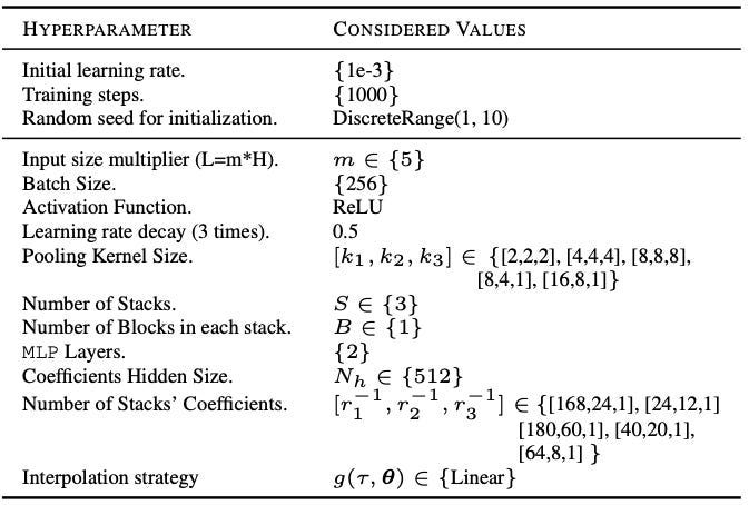
**Figure 12:** Hyperparameter tuning strategy of NHITS (*Source*)

Notice the Pooling Kernel Size k (which concerns Multi-Rate Sampling) and the Stacks' Coefficients 1/r1 (the expressiveness ratios of Hierarchical Interpolation)

Typically, these values are higher in the first stack and decrease over subsequent stacks, eventually reaching 1. Specifically:

Blocks in the 1st stack have large k and high 1/r ratios, producing low-frequency signals through aggressive interpolation. These blocks mostly learn long-term dependencies
In contrast, blocks in the final stack have smaller k and 1/r values (often 1), generating high-frequency data points.

Depending on your dataset and forecasting goals, you can adjust these parameters as needed:

**Figure 13**: *Probabilistic energy demand forecasting using NHITS (Image by author)*

**Figure 14:** *Monitoring Hyperparameter tuning of NHITs using Tensorboard (Image by author)*

Closing Remarks

NHiTS is a cutting-edge, proven model that excels in time-series forecasting.

What I like about NHiTS is that, with a few simple upgrades over its predecessor NBEATS, it achieves impressive results – while being more lightweight.

The key to top-performing deep learning models in time-series forecasting isn't just stacking hidden layers. Instead, they incorporate statistical concepts in a way that respects the unique properties of time-series data.

If you're interested in how Deep Learning models integrate these statistical principles to enhance performance, check out this comprehensive essay on deep learning forecasting models: