How Exactly Does a Decision Tree Solve a Regression Problem?

In this article, I'm going to demonstrate through a simple example, flowchart, and code – the entire logic implemented under the hood of a Decision Tree regressor (aka regression tree). After reading it, you will be able to get a clear idea behind the working of regression trees, and you will be more thoughtful & confident in using and tuning them in your next regression challenge.

We will cover the following:

• An awesome introduction to decision trees
• Generating a toy data set for training our regression tree
• Outlining the logic of the regression tree in the form of a flowchart
• Referencing the flowchart to write the code using NumPy and Pandas and make the first split
• Visualizing the decision tree after our first split, using Plotly
• Generalizing the code using recursion to build the entire regression tree
• Use scikit-learn to perform the same task and compare the results (spoiler: you'll be so proud that you produced the same output as scikit-learn did!)

Introduction

Decision trees are Machine Learning algorithms that can be used to solve both classification as well as regression problems. Even though classification and regression are inherently different from each other, decision trees try to approach both of these problems in an elegant way where the ultimate goal is to find the best split at a given node. And, how that best split is determined is what makes a classification tree and a regression tree different from each other.

In my previous article, I touched upon the basics of how a decision tree solves a classification problem. I used a two-class dataset to demonstrate a step-by-step process to understand how a decision rule is generated at each node using data impurity measures such as entropy, and then later implemented a recursive algorithm in Python to output the final decision tree. Not sure if you should add this article to your reading list? Let's use a decision tree to find out!

Important Note: This was just an example to show what a decision tree is, AND you're awesome no matter if it says that or not.

As shown above, a decision tree classifier aims to predict discrete labels (or classes) which in our case are You R Awesome! and Go READ IT!. In such cases, the decision tree looks at the probability distribution of the classes at each split to compute measures such as entropy and hence decides the best feature and value to split on.

However, in Regression problems, the target variable is continuous and we cannot use entropy (or Gini index) as the split criterion in such cases. So, regression trees make use of Mean Squared Error (MSE) and choose the feature and value that leads to the minimum MSE at each node.

Mean Squared Error: It is defined as the sum of squared differences between the true values and predicted values.

Building a Regression Tree

To demonstrate how a regression tree is learned, I'm going to use NumPy to generate a toy dataset resembling a quadratic function that will be used as the training data. Feel free to pause and bring up a new Python notebook on the side to code along as you read.

Let's import the libraries first.

import pandas as pd
import numpy as np
import plotly.graph_objects as go
import plotly.express as px

Generating the dataset

In the following code, we're going to generate the training data where our target i.e. dependent variable y is a quadratic function of independent variable X. For the sake of simplicity, I'm considering a single feature X, but it can be extended easily with multiple features (both continuous and categorical features).

Here, both X and y are continuous (y has to be continuous since it's regression and X could be either categorical or continuous).

# Set a random seed for reproducibility
np.random.seed(0)

# Constants for the quadratic equation
a, b, c = 1, 2, 3

# Create a DataFrame with a single feature
n = 100  # number of samples
x = np.linspace(-10, 10, n)  # feature values from -10 to 10
noise = np.random.normal(0, 10, n)  # some random noise
y = a * x**2 + b * x + c + noise  # quadratic equation with noise

# create a pandas dataframe
df = pd.DataFrame({'X': x, 'y': y})

Visualizing the data

We have created 100 data points. Let's use Plotly to visualize our data as follows.

df = data.copy()

# Create the figure
fig = go.Figure()

# Add scatter plot trace
fig.add_trace(
    go.Scatter(
        x=df["X"], 
        y=df["y"], 
        mode="markers", 
        marker=dict(opacity=0.7, size=6, color="red",
                    line=dict(color='Black', width=1))
    )
)

# Update layout
fig.update_layout(
    title={
        'text': "Scatter plot of our sample data",
        'y':0.9,
        'x':0.5,
        'xanchor': 'center',
        'yanchor': 'top'},
    xaxis=dict(
        title="X",
        showline=True,  # Show the X axis line
        tickmode='linear',  # Tick mode to be linear
        # tick0=-10,  # Start tick at 0
        dtick=1,  # Tick at every 1 unit
        linecolor='black',  # X axis line color
    ),
    yaxis=dict(
        title="y",
        showline=True,  # Show the Y axis line
        linecolor='black',  # Y axis line color
    ),
    plot_bgcolor='white',  # Background color
    width=900,
    height=500
)

# Show the figure
fig.show()

Cell Output:

Ready to make our first split?

Before doing that, let's first outline the steps a regression tree takes and then we will refer to these steps to write our code. Spending some time studying the flowchart below is all we need to do to understand the underlying logic of a regression tree to find the optimal split at a given node.

Once the above logic is clear, we are all set to witness the regression tree make its first optimal split using the following code.

We need to first define a helper function to calculate MSE.

def mean_squared_error(y, y_hat):
"""
Returns mean squared error for 
given actual values and predicted values
"""
  y = np.array(y)
  y_hat = np.array(y_hat)
  return np.mean((y-y_hat)**2)

The following code is the core logic as explained in the flowchart above.

df = data.copy()

# list of all features (only one i.e., 'X' in our case)
features = ["X"]

# iterate over all features
for feature in features:
  # initialize best_params dict
  best_params = {"feature": None, # best feature
                 "split_value": None, # best split value
                 "weighted_mse": np.inf, # weighted mse of two branches
                 "curr_mse": None, # mse at current node
                 "right_yhat": None, # prediction at right branch
                 "left_yhat": None # prediction at left branch
                 }
  # sort the df by current feature
  df = df.sort_values(by=feature)

  # compute the mse at current node
  curr_yhat = np.mean(df['y'].mean())
  curr_mse = mean_squared_error(df['y'], curr_yhat)
  curr_mse = np.round(curr_mse, 3)

  # iterate over all rows of sorted df
  for i in range(1, len(df)):
    # compute average of two consecutive rows
    split_val = (df.iloc[i][feature] + df.iloc[i-1][feature]) / 2
    split_val = np.round(split_val, 3)

    # split the df into two partitions
    left_branch = df[df[feature]<=split_val]
    right_branch = df[df[feature]>split_val]

    # compute the MSE of both partitions:

    left_yhat = np.mean(left_branch["y"]) # prediction will be average of target
    left_yhat = np.round(left_yhat, 3)
    left_mse = mean_squared_error(left_branch["y"], left_yhat) # mse of left
    left_mse = np.round(left_mse, 3)

    right_yhat = np.mean(right_branch["y"]) # prediction will be average of target
    right_yhat = np.round(right_yhat, 3)
    right_mse = mean_squared_error(right_branch["y"], right_yhat) # mse of right
    right_mse = np.round(right_mse, 3)

    # compute weighted MSE
    weighted_mse = ((len(left_branch) * left_mse) + (len(right_branch) * right_mse))/len(df)
    weighted_mse = np.round(weighted_mse, 3)

    # update best_params if weighted_mse is less than previously best_mse
    if weighted_mse <= best_params["weighted_mse"]:
      best_params["weighted_mse"] = weighted_mse
      best_params["split_value"] = split_val
      best_params["feature"] = feature
      best_params["curr_mse"] = curr_mse
      best_params["right_yhat"] = right_yhat
      best_params["left_yhat"] = left_yhat

best_params

Cell Output:

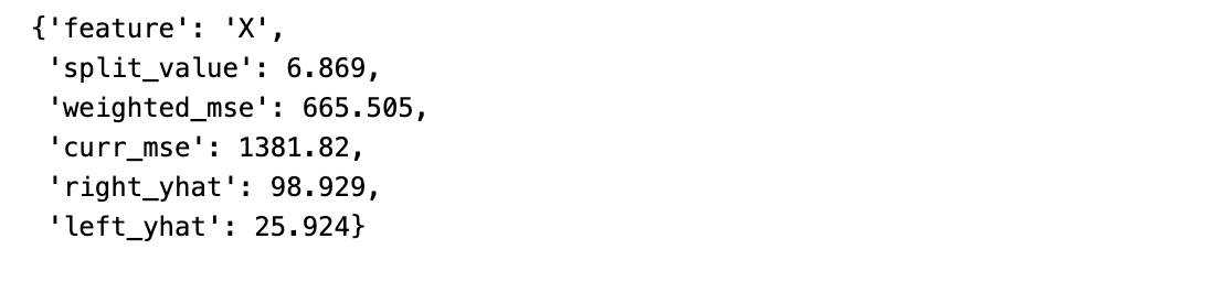
Yayy! We got our first optimal split at X=6.869. Let's visualize it as follows:

# add vertical line to existing figure
fig.add_vline(x=best_params["split_value"], line_width=3, line_color="black")

# plot right branch split
fig.add_shape(type="line",
x0=best_params["split_value"], y0=best_params["right_yhat"],
x1=10, y1=best_params["right_yhat"],  
line=dict(color="gray", width=3))

# plot left branch split
fig.add_shape(type="line",
x0=-10, y0=best_params["left_yhat"],
x1=best_params["split_value"], y1=best_params["left_yhat"],  
line=dict(color="gray", width=3))

# fig.update_layout(title=
fig.update_layout(
title={
    'text': f"X<={np.round(best_params["split_value"],2)}, MSE={np.round(best_params["curr_mse"],2)}, samples={len(df)}, value={np.round(df["y"].mean(),2)}",
    'y':0.9,
    'x':0.5,
    'xanchor': 'center',
    'yanchor': 'top'},
)

fig.show()

Cell Output:

Interpretation of the above result:

• X<=6.869 corresponds to the split value. It means that the data at the current node will get subdivided into two parts – one where X<=6.869 and the other where X>6.869. That's what the black vertical line represents.
• samples=100 corresponds to the total number of data points at the current node. Initially, the root node consists of all data points.
• MSE=1381.82 corresponds to the value of the mean squared error at this current node. We know that MSE needs true values and predicted values for its calculation; we already have true values, what are the predicted values you might be wondering, right? That's value.
• value=37.605 corresponds to the prediction at the current node. The prediction at any node is the average of all true values belonging to the data at the given node. Initially, prediction at the root node will simply be the average of y values of all 100 rows.
• The horizontal gray lines on both sides of the split represent the predictions for the left partition and right partition.

Optional exercise: Copy the two cells we used above and replace the original df with either of the left partition or right partition data frames. You can see how subsequent splits are being made for them in the exact same manner. Just the input data frame changes and everything else (the core logic) remains the same.

Following is how the current state of our regression tree looks like after repeating the code for the left and right branches:

I hope it makes it easier now to interpret a regression tree that looks like below:

The above process gets repeated for the subsequent partitions until a stopping criterion is met (such as max depth reached, no further splitting possible, etc.).

Generalize the code using recursion

Let's wrap the above code inside a function build_tree that we can call recursively to build the regression tree.

Helper functions:

mean_squared_error: Returns the mean squared error for the given actual values and predicted values. Defined above.

get_best_params: Returns the _bestparams dictionary that consists of the feature and value to use for splitting the data at the current node as well as contains the prediction for the current node.

def get_best_params(df):
"""Function to return best split"""
    for feature in features:
    # initialize best_params dict
        best_params = {"feature": None, # best feature
                 "split_value": None, # best split value
                 "weighted_mse": np.inf, # weighted mse of two branches
                 "curr_mse": None, # mse at current node
                 "right_yhat": None, # prediction at right branch
                 "left_yhat": None # prediction at left branch
                 }
        # sort the df by current feature
        df = df.sort_values(by=feature)

        # iterate over all rows of sorted df
        for i in range(1, len(df)):
            # compute average of two consecutive rows
            split_val = (df.iloc[i][feature] + df.iloc[i-1][feature]) / 2
            split_val = np.round(split_val, 3)

            # split the df into two partitions
            left_branch = df[df[feature]<=split_val]
            right_branch = df[df[feature]>split_val]

            # compute the MSE of both partitions:

            left_yhat = np.mean(left_branch["y"]) # prediction will be average of target
            left_yhat = np.round(left_yhat, 3)
            left_mse = mean_squared_error(left_branch["y"], left_yhat) # mse of left
            left_mse = np.round(left_mse, 3)

            right_yhat = np.mean(right_branch["y"]) # prediction will be average of target
            right_yhat = np.round(right_yhat, 3)
            right_mse = mean_squared_error(right_branch["y"], right_yhat) # mse of right
            right_mse = np.round(right_mse, 3)

            # compute weighted MSE
            weighted_mse = ((len(left_branch) * left_mse) + (len(right_branch) * right_mse))/len(df)
            weighted_mse = np.round(weighted_mse, 3)

            # update best_params if weighted_mse is less than previously best_mse
            if weighted_mse <= best_params["weighted_mse"]:
                best_params["left_yhat"] = left_yhat
                best_params["right_yhat"] = right_yhat
                best_params["weighted_mse"] = weighted_mse
                best_params["split_value"] = split_val
                best_params["feature"] = feature
                best_params["curr_mse"] = curr_mse

    return best_params

build_tree: It is the main driver function that utilizes helper functions to build the regression tree recursively. I have added parameters such as _maxdepth so that the growth of the regression tree can be controlled to avoid overfitting, and also to serve as a stopping criterion.

def build_tree(df, max_depth=3, curr_depth=0):
    """Function to build the regression tree recursively"""

    if curr_depth>=max_depth:
        prediction = np.round(np.mean(df["y"]), 3)
        print(("--" * curr_depth) + f"Predict: {prediction}")
        return

    best_params = get_best_params(df)

    if best_params["feature"] is None or best_params["split_value"] is None:
        prediction = np.round(np.mean(df["y"]), 2)
        print(("--" * curr_depth) + f"Predict: {prediction}")
        return

    feature = best_params["feature"]
    split_val = best_params["split_value"]

    # Print the current question (decision rule)
    question = f"{feature} <= {split_val}"
    mse = mean_squared_error(df["y"], df["y"].mean())
    mse = np.round(mse, 3)
    samples = len(df)
    print(("--" * (curr_depth*2)) + ">" + f"{question}, mse: {mse}, samples: {samples}, value: {np.round(df["y"].mean(),3)}")

    left_branch = df[df[feature]<=split_val]
    right_branch = df[df[feature]>split_val]

    # recursive calls for left and right subtrees
    if not left_branch.empty:
        print(("--" * curr_depth) + f"Yes ->")
        build_tree(left_branch, curr_depth=curr_depth+1)

    if not right_branch.empty:
        print(("--" * curr_depth) + f"No ->")
        build_tree(right_branch, curr_depth=curr_depth+1)

Now let's call the above function on our training data.

build_tree(data)

Cell Output:

The above output corresponds to the regression tree given max_depth=3. For more clarity, refer to the following diagram of our regression tree.

The leaf nodes in the above regression tree correspond to the prediction values. On plotting the predictions and decision boundaries as per our final regression tree, we will get something like this:

Link to Code

You can find the full notebook here.

The moment of truth – Implementing regression tree using scikit-learn and comparing the final tree with ours

Now we need to know whether our understanding of the working of regression trees is accurate or not. To do that, let's use scikit-learn to train a regression tree on the same data and look at the final results as follows.

from sklearn.tree import DecisionTreeRegressor
from sklearn import tree
import matplotlib.pyplot as plt

# Fit the regression tree
regressor = DecisionTreeRegressor(max_depth=3)
X = np.array(data["X"]).reshape(100, 1)
y = np.array(data["y"])
regressor.fit(X, y)

# Plot the tree
plt.figure(figsize=(15, 8))
tree.plot_tree(regressor, feature_names=['X'], filled=True)
plt.show()

Cell Output:

The regression tree returned by scikit-learn's DecisionTreeRegressor is the exact same as the one we created previously.

Not a mystery anymore!

I hope that staying so far in this article has been valuable for you and hopefully this one line of code i.e., regressor.fit(X, y) is no longer a mystery. Since we are now well aware of how the underlying algorithm has been fabricated, we can be more thoughtful while tweaking our tree-based regression models in the future.

This is not the end

The purpose of this article was to solely demonstrate the logic used by a decision tree regressor to make the optimal split at a node. However, it's not a comprehensive guide on decision trees since there are many other important aspects that also need to be taken care of while modeling. It will be unfair if we don't discuss them at all, so providing a brief summary of some points here.

Advantages of decision trees:

• Decision trees are interpretable and intuitive since one can get a clear idea of what led to a specific prediction.
• They do not demand much preprocessing of the training data, and can intrinsically handle categorical features and missing values.

Disadvantages of decision trees:

• Decision trees are sensitive to small variations in the data.
• When not controlled properly, decision trees are highly prone to overfitting, and suitable measures need to be taken to prevent the tree from overgrowth so that they generalize well.

Conclusion

In this article, we learned to build a regression tree from scratch to thoroughly understand the logic behind it. We generated a simple dataset with one continuous feature X and target y, that was used to train the decision tree regressor. It was followed by communicating the approach taken by the regression tree at each node to determine the best split via a flowchart so that it is easier for us to write code with having clear picture of the sequence of steps. We visualized the first best split returned by the code and discussed how the same logic can be extended further to build the entire tree.

We also trained a decision tree regressor using scikit-learn on the same data and noticed that it produced the same results as we did previously from scratch. The goal of this article was to look at what exactly is going on in the backend when we call .fit() on our data to train a DecisionTreeRegressor model from scikit-learn.

Hopefully, having this knowledge is going to help us better tweak, tune, and interpret our tree-based regression models in the future.

---

Thank you for reading

Tags: Data Science Decision Tree Getting Started Machine Learning Regression

Comment