How to Low-Pass Filter in Google BigQuery
When working with time-series data it can be important to apply filtering to remove noise. This story shows how to implement a low-pass filter in SQL / BigQuery that can come in handy when improving ML features.
Filtering of time-series data is one of the most useful preprocessing tools in Data Science. In reality, data is almost always a combination of signal and noise where the noise is not only defined by the lack of periodicity but also by not representing the information of interest. For example, imagine daily visitation to a retail store. If you are interested in how seasonal changes impact visitation, you might not be interested in short-term patterns due to weekday changes (there might be an overall higher visitation on Saturdays compared to Mondays, but that is not what you are interested in).
time-series filtering is a cleaning tool for your data
Even though this might look like a small issue in the data, noise or irrelevant information (like the short-term visitation pattern) certainly increases your feature complexity and, thus, impacts your model. If not removing that noise, your model complexity and volume of training data should be adjusted accordingly to avoid overfitting.

This is where filtering comes to the rescue. Similar to how one would filter outliers from a training set or less important metrics from a feature set, time-series filtering removes noise from a time-series feature. To put it short: time-series filtering is a cleaning tool for your data. Applying time-series filtering will restrict your data to reflect only the frequencies (or timely patterns) you are interested in and, thus, results in a cleaner signal that will enhance your subsequent statistical or machine-learning model (see Figure 1 for a synthetic example).
What is a Filter?
A detailed walkthrough of what a filter is and how it works is beyond the scope of this story (and a very complex topic in general). However, on a high level, filtering can be seen as a modification of an input signal by applying another signal (also called kernel or filter function) to it.
Since the key purpose of a filter is to restrict the data to a certain pattern (and so remove the pattern representing noise), it is essential to ensure the kernel is designed in a way that it resonates with the signal that is worth keeping (the signal of interest). After successfully defining the kernel, the combination of the original input signal and the kernel will provide the cleaned version of the signal (a process called convolution).
It is important to highlight that this combination between signal and kernel can be either applied as a windowed function or via a Fourier transformation. Since the implementation of a Fourier transformation requires complex numbers, which are to date not natively supported in Google Bigquery, this story will focus on the first approach using a windowed function.
Put short and very simplified: a time-series filter can also be seen as just a time-wise multiplication of an input signal with a pre-defined kernel.
Why Filtering Features for Machine Learning?
As mentioned above, allowing for a lot of noise in input features to a machine learning model is not recommended. Noise will harm the data quality and, thus, have an immediate impact on the resulting model (garbage in, garbage out).
However, even when additional time-series patterns are not strictly noisy but represent a mixture of different information, it can be good practice to separate that information into different features for many reasons:
- Feature Importance: Separation allows the investigation of feature importance and model explainability separately per time-series information. Daily variability could be more or less important than seasonality. But without splitting that information into separate features, it will be challenging to investigate.
- Sensitive Loss Function: Ensure the model learns what it is supposed to learn. If the aim is to train a model predicting the seasonal impact on the retail market, you might want to remove any daily variance from the features. Otherwise, the loss function might be sensitive to the daily variance and update weights based on the wrong information.
- Overfitting: Even though it is so easy to just provide more features or increase model complexity to handle complex input features, it should be good practice to focus on Feature Engineering first to prevent overfitting.
Example Use Case: Predict Restaurant Visitation
To provide a real-world application of filtering, we will take the use case to build a model that predicts restaurant visitation (Figure 2). When thinking about this use case in the US, there might be a correlation between certain food type consumption and the seasonal temperature. Therefore, weather data could be a potential predictor of restaurant visitation (among a lot of other features).

However, weather data consists of both, long-term (climate) and short-term (weather) data. Depending on your detailed modeling approach, applying filtering and removing the short-term patterns in your data might be beneficial.
Implement a Windowed Filter in Google BigQuery
Now that we have defined a potential use case, we will go step-by-step through how to fetch data, define a filter, and apply filtering in Google Bigquery.
1. Fetch Weather Data
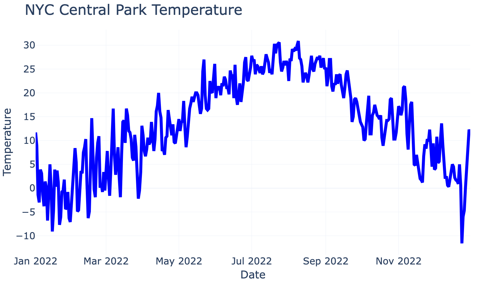
The first step is to source weather data. You can source any data you are interested in. For simplicity, here we will fetch weather data that is publicly available in BigQuery (see code below). To do so, we define the time range and location for which we would like to source weather data. The query below shows how easy fetching that data can be and Figure 3 plots the resulting average temperature for the year 2022 for New York City Central Park. Please keep in mind that a detailed walkthrough of the code below is beyond the scope of this story since it "just" fetches example data.
DECLARE
  input_year INT64 DEFAULT 2022; -- time
DECLARE
  location STRING DEFAULT "NY Central Park"; -- name
DECLARE
  geom GEOGRAPHY DEFAULT ST_GEOGPOINT(-73.974282, 40.771464); -- location

WITH
-- Fetch weather stations that have > 360 days with temperature recorded in the US.
  stations_with_data AS (
  SELECT
    id,
    COUNT(DISTINCT
      CASE WHEN element = "TMAX" THEN date ELSE NULL END
    ) tmax_date_n
  FROM
    `bigquery-public-data.ghcn_d.ghcnd_stations`
  JOIN
    `bigquery-public-data.ghcn_d.ghcnd_*` USING(id)
  WHERE
    qflag IS NULL
    AND element IN ('TMIN','TMAX')
    AND _TABLE_SUFFIX = CAST(input_year AS STRING)
    AND value IS NOT NULL
  GROUP BY id
  HAVING (tmax_date_n >= 360) ),

-- calculate the linear distance between the location of interest (NYC Central Park) and each weather station.
  calc_distance AS (
  SELECT
    s.id,
    location,
    s.state,
    ST_DISTANCE(geom, ST_GEOGPOINT( s.longitude, s.latitude)) AS distance
  FROM
    `bigquery-public-data.ghcn_d.ghcnd_stations` s
  JOIN
    stations_with_data USING(id)
  WHERE
    ST_DWITHIN(geom, ST_GEOGPOINT( s.longitude, s.latitude), 10000) ),

-- pick closest weather station
  fetch_closest AS (
  SELECT
    location,
    ARRAY_AGG(STRUCT(id,
        state,
        distance)
      ORDER BY distance
      LIMIT 1) station
  FROM
    calc_distance
  GROUP BY 1 ),

-- Unnest station and transform distance to KM
  unnest_closest AS (
  SELECT
    location,
    id,
    CAST(distance / 1000 AS INT64) distance_km
  FROM
    fetch_closest, UNNEST(station) ),

-- fetch weather data only for the closest station
  get_weather AS (
  SELECT
    location,
    date,
    IF(element = 'TMIN', value, NULL) AS tmin,
    IF(element = 'TMAX', value, NULL) AS tmax
  FROM
    `bigquery-public-data.ghcn_d.ghcnd_*`
  JOIN unnest_closest USING(id)
  WHERE
    qflag IS NULL
    AND element IN ('TMIN','TMAX')
    AND _TABLE_SUFFIX = CAST(input_year AS STRING) )

-- take average between min() and max() and divide by 10 to get average daily temperature in Celsius
SELECT
  location,
  date,
  CAST((MAX(tmin) + MAX(tmax)) / 2 AS INT64) / 10 AS avg_temp
FROM
  get_weather
GROUP BY location, date
Even though this code is quite long, it simply fetches some data we want to filter (here: data for the closest weather station to NYC Central Park for the year 2022) and does some transformation to it (create average temperature per day). If you have your own data you want to filter, you can just ignore this code and move on with your data.
2. Define Filter Function
Now that we have data that we want to filter, we need to define the Kernel/filter function. Unfortunately, BigQuery does not natively support complex numbers which makes a more useful implementation of a filter using Fourier and inverse Fourier transformation very complicated. However, as we learned before, it is possible to implement a filter using a windowed function with real numbers. Hence, we will define a Kernel in the form of a Hann window as follows:
CREATE TEMP FUNCTION HANN(x float64) AS
(0.5 * ( 1 - COS(( 2 * ACOS(-1) * x) / ( 28 - 1 ))));
This code defines a temporary function called "Hann" that takes an input value x and transforms it into its representation of a Hann window of the length 28. You must adjust the 28 here if you are interested in a different filter length or parameterize that input, too. The remaining math follows the formula for the Hann window (fetched from Wikipedia).
3. Apply Filter
Now that we have data we want to filter and we have a filter function defined (the Kernel above), we can put all of this together and create a windowed function that multiplies the Kernel with the data similar to a moving average (just weighted by the Hann function). Figure 4 shows the result of the code below when the Hann window is applied to the weather data and that it will result in a smoothed line representing more long-term weather trends.
--define hann gaussian with 28 window length
CREATE TEMP FUNCTION
  HANN(x float64) AS (0.5 * ( 1 - COS(( 2 * ACOS(-1) * x) / ( 28 -1 ))));

WITH
-- fetch the weather data as shown before
  weather_data AS (
  SELECT
    location,
    date,
    avg_temp
  FROM
    `your_project.your_dataset.your_weather`
  GROUP BY location, date, distance_km ),

-- create kernel/filter function and standardise
  set_kernel AS (
  SELECT
    HANN(k) / SUM(HANN(k)) OVER() AS kernel,
    ROW_NUMBER() OVER() AS idx
  FROM
    UNNEST(GENERATE_ARRAY(0,27)) AS k ),

-- add row number per date to apply window function later
  add_row_number AS (
  SELECT
    date,
    avg_temp,
    ROW_NUMBER() OVER(ORDER BY date) idx
  FROM
    weather_data
  GROUP BY date, avg_temp ),

-- apply a window function (of length 28) to every single date across previous and following dates
  apply_window_function AS (
  SELECT
    date,
    ARRAY_AGG(STRUCT(date AS t, avg_temp)) OVER w1 AS v
  FROM
    add_row_number
  WINDOW
    w1 AS (
    ORDER BY idx ROWS BETWEEN 14 PRECEDING AND 13 FOLLOWING) ),

-- unnest that huge vector created by the window function for subsequent multiplication
  unnest_vector AS (
  SELECT
    date,
    t,
    avg_temp,
    ROW_NUMBER() OVER(PARTITION BY date ORDER BY t) AS idx
  FROM
    agg, UNNEST(v) )

-- final multiplication of each window with kernel to apply the filtering and sum up to get the final data
SELECT
  date,
  SUM(avg_temp * COALESCE(kernel, 0)) AS smooth_line
FROM
  t
LEFT JOIN set_kernel USING(idx)
GROUP BY date
Even though the code above looks quite complex, it actually performs a fairly straightforward multiplication via a windowed function. As a first step, it only fetches the data. First, the weather data, and second it creates the filter function. Then, to be able to apply the windowed function per date later, we create an index based on the row_number ordered by the date.
After that preprocessing is done, we can apply the windowed function that creates for every date a window of the preceding 14 and the following 13 days. Basically, for every day it creates a vector corresponding to the kernel length (the Hann window). As the very last step, the kernel is multiplied with each vector for each day and summed up resulting in the smoothed/filtered signal as shown in Figure 4.
Conclusion
In most of the cases, Data Scientists are not working with clean data. It is more common that the data to work with is superimposed of the signal of interest and some form of noise. Cleaning that data can enhance subsequent statistical and machine-learning models.
As shown above, cleaning time-series data using a filter in Bigquery is feasible and extremely powerful and provides a workaround if a Fourier transformation is not possible. In addition, this filtering has a very short runtime and is fairly scalable. The resulting signal represents less noise and more signal of interest and, thus, reduces feature complexity and overfitting of any subsequent modeling approach.
All images, unless otherwise noted, are by the author.
Please check out my profile page, follow me, or subscribe to my email list if you would like to know what I write about or if you want to be updated on new stories.
