How to Select the Most Influential Combination of Nodes in a Graph

When finding influential nodes in a graph, you can consider graph metrics such as centrality or degree, which tell you how influential a single node is. However, to find the most influential set of nodes in the graph, you must consider which combination of nodes has the highest influence on the graph, which is a challenging problem to solve. This article explores how you can approach the issue of choosing the most influential set of nodes from a graph.

Motivation

My motivation for this article is that I am currently working on my thesis, which involves semi-supervised clustering. In essence, I have to select some nodes from the graph that I can know the label of and then use that information to cluster the other nodes. Therefore, finding the most influential set of nodes to know the label is essential for the performance of my clustering algorithm. In this article's case, influence over the graph will be regarded as how well the set of selected nodes can assist the clustering algorithm. However, this influence over the graph can also be generalized to other problems.

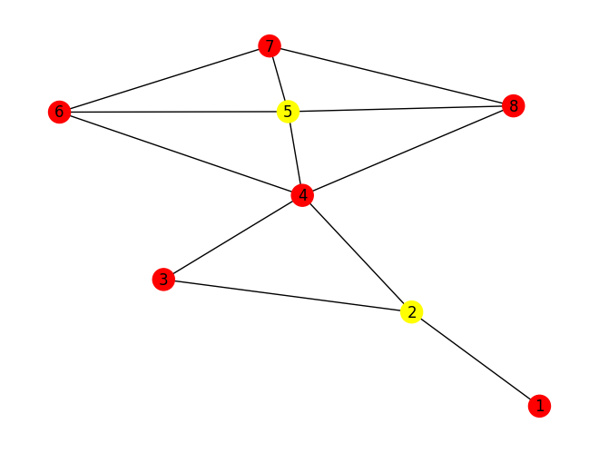
The problem of finding the most influential combination of nodes is interesting because, besides using an individual score for the node influence, you must also consider a node's position in the graph relative to other selected nodes. Selecting the combination of the most influential nodes makes the problem much more complicated since simply selecting the nodes with the highest individual influence score might not be optimal. This is illustrated in the figure below, where the two most influential nodes individually measured by degree are nodes 4 and 5. Choosing these two nodes, however, will not necessarily be the best option for influence over the whole graph. In this case, the two nodes are connected, and other combinations of nodes can, therefore, have a more substantial combined influence on the graph, like, for example, nodes 2 and 5, since those two nodes can directly reach all other nodes in the graph.

In this article, I will first discuss finding the influence of individual nodes by using different node influence metrics and show you ways to combine the metrics. Following that, I will show you heuristics for selecting combinations of nodes in the graph that significantly influence the graph. Then, I will combine the two techniques and choose combinations of nodes based on each node's influence and the combined influence of the combination of nodes. This will allow you to select a powerful combination of nodes in a network with the highest influence over the network.

Table of Contents

· Motivation · Table of Contents · Metrics for node influence · Combining metrics ∘ Normalize and add ∘ Select nodes separately for each metric · Choosing a set of nodes ∘ Using community detection ∘ Using a minimum number of steps between nodes ∘ Combining community detection and min number of steps · Testing the influence of the selected nodes ∘ Test 1: The number of nodes connected to chosen nodes ∘ Test 2: The number of communities connected to chosen nodes ∘ Test 3: Downstream tasks ∘ Test 4: Visual inspection · Conclusion

Metrics for node influence

Node influence is a general term for a node's significance within a graph. There exists many metrics for measuring this node influence, with some of the most common metrics being:

• Degree
• Betweenness centrality
• Closeness centrality
• Eigenvector centrality
• Infection spreading speed, inspired by the SIR model

The simplest metric to understand is the degree metric, which measures the amount of edges going in and out of a node. The more edges connected to a node, the more influential the node is. In social networks, you will typically see a graph following the power law, meaning that a few nodes are connected to many nodes, while most nodes are connected to a few nodes. This means that high-degree nodes tend to be connected to low-degree nodes. You can see this illustrated in the image below, with the blue histogram plot having a few nodes with a high degree and more nodes with a lower degree. On the other hand, you have more balanced graphs, with nodes of equal degrees being connected. This is illustrated in the yellow histogram plot, which follows a normal distribution.

Betweenness centrality is another common metric you can use. The betweenness centrality finds the shortest path between all pairs of nodes and counts how many shortest paths pass through each node. If many shortest paths pass through a node, that node is regarded as having a higher influence. Closeness centrality is measured in a similar way to betweenness centrality, but it measures more how close each node is to other nodes in the network. I also mentioned eigenvector centrality, which, in short terms, measures how well a node is connected to other well-connected nodes.

Lastly, the fourth metric I mentioned is the infection spread model, which is inspired by the SIR model. This model effectively measures how well a disease will spread, starting from each node. If the disease spreads quickly from a node, this indicates the node is more influential. You can read more about the infection spread model in my article on advanced graph analytics.

Which metric you should use would depend on the problem you are working on and your Graph type. It is usually difficult to know beforehand which metric best represents your graph, so testing the different metrics on a downstream task is often the way to go. Furthermore, as I will explain in the next section, you can also combine the different metrics to form a more powerful metric representing the influence of the nodes.

Combining metrics

In addition to calculating individual metrics for node influence, you can also combine the metrics together. I will show you two main approaches to combining the metrics in the graph. I will also visualize the chosen nodes in the graph, which you can do with the following function:

def highlight_frozen_nodes(G, freezed_nodes):
    """given adjacency matrix and a list of frozen nodes. Visualize a graph were the frozen nodes are highlighted. Graph is also drawn deterministically, so layout does not change everyti,e"""
    colors = ['yellow' if node in freezed_nodes else 'lightblue' for node in G.nodes()]
    pos = nx.spring_layout(G, seed=28)  # Fixed seed for reproducibility
    nx.draw(G, pos, with_labels=True, node_color=colors)
    plt.show()

Normalize and add

Firstly, you can simply add the two different metrics together in order to form a combined metric. When doing this, however, you must remember to normalize each metric to be between 0 and 1 first so the scale of the metrics is equal. The reasoning for this can be understood by looking at the two metrics, degree influence, and betweenness centrality influence. The degree for a node will typically range from 0 to a large integer, while the betweenness centrality will be between 0 and 1. If you combine the two numbers from different scales together, the larger number (in this instance the degree), will have a much larger impact. Thus, you have to remember to normalize the metrics before adding them together. You can see how to do this for the two node influence metrics degree and betweenness centrality below:

degrees = np.array(list(degree for _, degree in list(G.degree())))
centralities = np.array(list(nx.betweenness_centrality(G).values()))

# # normalize degree and centralities to be between 0 and 1
degrees = (degrees - np.min(degrees)) / (np.max(degrees) - np.min(degrees))
centralities = (centralities - np.min(centralities)) / (np.max(centralities) - np.min(centralities))

combined_scores = degrees + centralities
combined_scores

Naturally, this is not limited to two metrics, you can combine as many as you prefer, as long as each metric is normalized. Furthermore, you can also add weighting to each metric, which essentially says that some metrics are more important than others. If you, for example, regard the degree of a node to be of more importance for the influence of that node, you can add weighting to the degree metric to make that more important for a node's influence. You can see in the code below how I made the degree twice as important as betweenness centrality in the code below.

weighting = np.array([2/3, 1/3]).reshape(1, -1)
#normalize weighting to sum to 1:
weighting = weighting/np.sum(weighting)

degrees = np.array(list(degree for _, degree in list(G.degree())))
centralities = np.array(list(nx.betweenness_centrality(G).values()))

# # normalize degree and centralities to be between 0 and 1
degrees = (degrees - np.min(degrees)) / (np.max(degrees) - np.min(degrees))
centralities = (centralities - np.min(centralities)) / (np.max(centralities) - np.min(centralities))
combined_scores = np.column_stack((degrees, centralities))
# multiply by weights
weighted_combined_scores = combined_scores * weighting
# sum the weighted scores
summed_scores = np.sum(weighted_combined_scores, axis=1)

Select nodes separately for each metric

You can also choose to select nodes separately for each metric. Say you,, for example,, want to choose the N most influential nodes from a graph; you can first choose N/2 nodes from the degree metric and then choose N/2 nodes from the betweenness centrality metric. This alternative allows you to focus on only the degree and sometimes only on the betweenness centrality, which can be a strength if you value each individual more, not the combination of the two metrics. You could, for example, have a node with a very high degree that you want to choose, but if the node has a low betweenness centrality, it will not be chosen. However, selecting nodes separately for each metric will deal with this problem and allow you to select nodes if they perform well on a single metric.

Choosing a set of nodes

After you have calculated the node influence metric individually for each node, it is time to choose a node selection strategy. With this, I mean choosing the set of nodes that best represents the graph. This is a more difficult challenge to solve, as there are endless options for combinations of nodes you can pick. Thus, you need a heuristic that tells you how to make decisions about which nodes to include and exclude from your chosen nodes. Below, I will show you two main approaches to selecting a set of nodes that together best represent the graph, also taking the previously calculated node influence metrics into account.

Using community detection

The first approach you can use is community detection to find which communities each node belongs to. Several community detection methods like Louvain, Girvan-Newman, or Spectral clustering can be used. Which one you should use will depend on the problem you are working on. If you, for example, are working with weighted edges, I recommend using a community detection algorithm that considers the edges, like Louvain. Similarly, if you are working on a problem with a set number of communities, I also recommend choosing an algorithm that can use a set number of communities, like Spectral clustering.

I would also like to add that I am working on a semi-supervised clustering problem myself, but I still think the community detection approach to choosing a combination of nodes can be effective. The reasoning is that you do not need the community detection algorithm you are using to work flawlessly. The point of using community detection is finding nodes from different communities in the graph, which in turn will increase the representativeness of the combination of chosen nodes.

To select the set of most influential nodes, I would then first start by calculating the relevant node influence metrics for each node. I would then iterate over each community found by the community detection algorithm and choose the node with the highest node influence score within that community. Additionally, you have to make sure you are choosing nodes you have not chosen before. After choosing a node from the community, you can then move on to the next community and pick the most influential node from that community, and so on, until you have chosen a node from each community. You can then restart the loop at the first community and choose the second most influential node from that community. When you have picked the number of nodes you need, you exit the loop.

This method guarantees that you choose both high-influence nodes according to your own metrics and a varied sample of nodes from different communities. This will better represent the graph than only looking at the highest-influence nodes and ignoring all communities.

To do this in Python, you need the Python Louvain package:

pip install python-louvain

You can then use the code below to select nodes from each community based on the degree score for each node:

import community as community_louvain
# select one node per partition
def select_nodes_based_on_communities(G, partition, scores, n=2):
 """given a node influence score per node, select n nodes based on communities"""

 sorted_node_indices = np.argsort(scores)[::-1]   # highest to lowest degree node indices
 chosen_nodes = set()
 for _ in range(n):
  for community in set(partition.values()):
   for node_idx in sorted_node_indices:
    node_idx += 1 # node indices are 1-based
    if node_idx not in chosen_nodes and partition[node_idx] == community: 
     chosen_nodes.add(node_idx)
     if (len(chosen_nodes) >= n):
      return chosen_nodes
     break

 raise Exception("Not enough nodes to select") #if you got here, you did not select enough nodes

num_nodes_to_select = 2
partition = community_louvain.best_partition(G) 
selected_nodes = select_nodes_based_on_communities(G, partition, degrees, num_nodes_to_select)

Using the code above will choose nodes 4 and 5 from the graph, which are from different communities, as you can see in the image below:

The image above highlights an issue: even though the nodes are from different communities, they are often directly connected in the graph. In the next section, I will show you an approach that avoids this issue.

Using a minimum number of steps between nodes

Another approach you can use is ensuring a minimum number of steps between nodes. The simplest way to do this is to set the minimum number of steps to 2, which ensures that the chosen nodes are not neighbors.

To select the set of the most influential nodes, you first find all relevant node influence metrics for each node. You then select the most influential node according to your metrics. Next, you move on to the second most influential node. If that node is within the minimum number of steps of the already chosen node (in this case, if the second most influential node neighbors the most influential node), you ignore the node and move on to the third most influential node. If the third most influential node is more than 2 steps away from the already chosen node, you select that node.

You then continue like this, always ensuring that the newest chosen node is a minimum number of steps from all other chosen nodes. This ensures that your selection of nodes is a varied sample from the graph.

To do this with code, you can use the Python code below:

import community as community_louvain
# select one node per partition
def select_nodes_based_on_min_steps(G, scores, n=2, min_steps=2):
    """given a node influence score per node, select n nodes based on communities"""

    sorted_node_indices = np.argsort(scores)[::-1]   # highest to lowest degree node indices
    chosen_nodes = set()

    for _ in range(num_nodes_to_select): # run max num_nodes_to_select times. Use this loop to ensure we select from each community
        for n in range(n, 0, -1): # if we do not get all nodes to select in n steps, we will decrease n by 1 and try again
            for node_idx in sorted_node_indices: # iterate over nodes in order of score
                node_idx += 1 #since my nodes start at index 1
                if (node_idx not in chosen_nodes):
                    #check if node is at least n steps away from any frozen node
                    if all([nx.shortest_path_length(G, node_idx, chosen_node) >= n for chosen_node in chosen_nodes]):
                        chosen_nodes.add(node_idx)
                        if len(chosen_nodes) >= num_nodes_to_select:
                            return chosen_nodes

num_nodes_to_select = 2
min_steps = 2
selected_nodes = select_nodes_based_on_min_steps(G, degrees, num_nodes_to_select, min_steps)

Which will result in choosing the nodes 4 and 7, as you see in the image below:

Combining community detection and min number of steps

The third approach to choosing a combination of nodes is combining the two previous approaches I have talked about. First, you find the different communities in the graph. Then you can select the most influential nodes from each community, under the additional condition that the chosen node is also a minimum number of steps from the already chosen nodes.

In my opinion, this approach is the best way to select a combination of nodes. It ensures that each community in the graph is represented by a chosen node and further assures that the chosen nodes are not connected, which increases their representativeness.

Still, it is important to note that different approaches can work better or worse on different kinds of graphs. Which approach works best for you will depend on the graph you are using, and I therefore recommend trying out the different approaches to see which one works best for you.

You can choose a set of nodes based on both community detection and the minimum number of steps with:

def select_nodes_based_on_communities_and_min_number_steps(G, partition, scores, n=2, min_steps=2):
 """given a node influence score per node, select n nodes based on communities"""

 sorted_node_indices = np.argsort(scores)[::-1]   # highest to lowest degree node indices
 chosen_nodes = set()
 for _ in range(n):
  for community in set(partition.values()):
   for node_idx in sorted_node_indices:
    node_idx += 1
    if node_idx+1 not in chosen_nodes and partition[node_idx] == community and all([nx.shortest_path_length(G, node_idx, chosen_node) >= n for chosen_node in chosen_nodes]):
     chosen_nodes.add(node_idx)
     if (len(chosen_nodes) >= n):
      return chosen_nodes
     break

num_nodes_to_select = 2
min_steps = 2
partition = community_louvain.best_partition(G) 
selected_nodes = select_nodes_based_on_communities_and_min_number_steps(G, partition, degrees, num_nodes_to_select, min_steps)

This is essentially the same code as the community selection code but with another condition in the if statement, saying nodes have to be at least n steps apart.

If you use the code above, you should select the nodes 2 and 5, which will give the following result:

Testing the influence of the selected nodes

After you have selected nodes based on the node influence metrics and the community detection or minimum number of steps approach, you should also test them. The problem in this case is that there is no ground truth that can tell you if you have chosen the optimal set of nodes. Still, I will show you three tests you can use to gauge the quality of your chosen set of nodes.

Test 1: The number of nodes connected to chosen nodes

The first test calculates the number of nodes connected to your chosen nodes. This test represents how well your nodes are connected in the graph and can tell you if your combination of chosen nodes is representative of the graph. A higher score for this test will mean you have chosen a better set of nodes.

You should, however, be aware that this test will perform better if you prioritize choosing high-degree nodes since they will be connected to more nodes in general. Still, it is a good test to measure if using community detection or a minimum number of steps is the best way to choose a set of nodes for your graph. Additionally, you should use this test as a relative measure, only comparing it against other graphs on the same test to see if a graph is better or worse.

If you apply this test with the degree influence score and choose a combination of nodes with the community detection and a minimum number of steps, you select 8/ 8 nodes in the graph, which you can visualize like:

If you instead only selected nodes based on their community, you would be connected to 7 / 8 nodes in the graph, missing the node with index 1, as you can see in the image below:

Test 2: The number of communities connected to chosen nodes

Another test you can use is the number of communities hit by your chosen set of nodes. This test can represent how well your chosen set of nodes affects the different communities in the graph, which is important for reaching all nodes in the graph. You should note, however, that this test will naturally be biased toward choosing a set of nodes based on their community. This test should also be used as a relative measure, similar to the last test I explained.

Test 3: Downstream tasks

Another solid test you can use is testing the chosen nodes on a downstream task. For example, I am using the set of chosen nodes for a semi-supervised clustering downstream task. I can, therefore, test out different approaches to selecting the nodes.

However, it is important to remember that when testing on downstream tasks, several other factors can come into play, like stochasticness in the clustering or other decisions like hyperparameters. Still, the scores achieved on the downstream tasks can indicate the quality of the chosen nodes.

Test 4: Visual inspection

The fourth and last test is the visual inspection, which is a test I always recommend doing when working on a Machine Learning project. Doing a visual inspection will allow you to understand the problem you are working on further. In this case, doing a visual inspection of the chosen nodes allows you to see the influence the chosen nodes have on your graph, and especially for smaller graphs; you can understand if the set of chosen nodes is good or bad. If you, for example, notice that a lot of outlier nodes are selected during the visual inspection, this indicates that your node selection has a bug in it, which you need to fix. Furthermore, the visual inspection also allows you to spot potential improvements in how you select your set of nodes.

When visually inspecting the nodes, I used a lot of NetworkX for smaller graphs, which allowed me to visualize the graph directly in my Jupyter Notebook. This does not work too well for larger graphs, however, in which case, I recommend using a graph visualization tool like Cytoscape, which has a plethora of options for visualizing your graph and looking into interesting aspects of the graph, which can help you gain further understanding of your graph. If you want to learn more about understanding the quality of your graphs, you can read my article below:

How to Test Graph Quality to Improve Graph Machine Learning Performance

Conclusion

In this article, I have talked about different approaches you can use to select the most influential combination of nodes in a graph. First, you calculate the influence of each node individually using metrics like degree or betweenness centrality. You can then use different approaches to select a combination of nodes, like selecting nodes from different communities with community detection algorithms like Louvain. You can also select nodes with a minimum number of steps between them or use a combination of a minimum number of steps and community detection. Finally, I have also mentioned four different tests you can use to test the quality of your chosen nodes, with the tests:

1. The number of nodes connected to chosen nodes
2. The number of communities connected to chosen nodes
3. Downstream tasks
4. Visual Inspection

You can also read my articles on WordPress.

Tags: AI Data Science Graph Hands On Tutorials Machine Learning

Comment