Implementing Simple Neural Network Backpropagation from Scratch
Why I Wrote This Article:
I've been using machine learning libraries a lot, but I recently realized I hadn't fully explored how Backpropagation works.
Understanding the fundamentals is crucial for keeping up with the latest technologies and identifying bugs in machine learning projects.
In this article, I share my experience building a simple neural network from scratch using just NumPy, and I compare its performance against PyTorch implementations. This will give you a hands-on understanding of fundamental concepts behind backpropagation.
Outline
・Introduction to the XOR Gate Problem
・Constructing a 2-Layer Neural Network
・Forward Propagation
・Chain Rules for Backpropagation
・Implementation with NumPy
・Comparing Results with PyTorch
・Summary
・References

Introduction to the XOR Gate Problem
The XOR (exclusive OR) gate problem is considered simple for a neural network because it involves learning a simple pattern of relationships between inputs and outputs that a properly designed network can capture, even though it is not linearly separable (meaning you can't draw a single straight line to separate the outputs into two groups based on inputs). Neural Networks, particularly those with hidden layers, are capable of learning non-linear patterns. Let's look at the inputs and outputs of XOR Gate. Here is our 4 training data.

Constructing a 2-Layer Neural Network
we use the most simple 2-layer fully connected Neural Network as an example to solve the XOR Gate problem. Here is the structure of this network. The input layer has j nodes, j = 2 in our case. the hidden layer has i nodes, i = 4. The output layer has k nodes, k = 1.

Forward Propagation: Key Concept: Matrix Calculations!
Understanding Training Data and Network Parameters: The input Data x is represented by a matrix of (2,4). This format is used because we have 4 training examples , and each example comprises2 inputs.

The weights between the layers are w¹ and w². Here w¹ is a matrix with dimensions of (i, j) and w² is a matrix of dimensions of (k, i). The biases for each layer, b¹ **** and b², play an important role in the neural network by introducing a slight offset within the activation function to provide additional flexibility. _b¹ has dimensions (i, 1)_ and _b² has dimensions (k,1_). The choice of _b¹ ‘s dimensions as (i, 1) instead of (j, i_) is deliberate to minimize the number of parameters, thereby simplifying the model without compromising its effectiveness. Activation function: I used the sigmoid function here.
The math equations of Feedforward Propagation are as follows:

The difference between the network's prediction and the actual answer is calculated through a loss function. This error measures how ‘off' the network's guess was. I use cross-entropy loss as the loss function because the XOR Gate problem is a binary classification problem.

where N is the number of training data, N=4, y represents the true label and a² is the network's output.
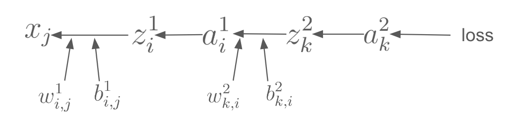
Chain rules for backpropagation
What is backpropagation? Once you get the error (loss), the algorithm works backwards from the output layer (where the prediction was made) to the input layer, calculating how much each part of the network (each node) contributed to the error. It does this by using calculus, specifically the chain rule, to find the gradient of the error function with respect to each weight in the network.
What are Chain rules? If a variable z depends on the variable y, which itself depends on the variable x, then z depends on x as well, via the intermediate variable y. In this case, the chain rule is expressed as follows:

An Example of the Chain Rule: Does the concept of multiplication in this context make sense to you? Let's consider a more intuitive explanation of the chain rule: If a car travels twice as fast as a bicycle, and the bicycle is four times as fast as a walking man, then the car travels 2 × 4 = 8 times as fast as the man. This analogy offers an intuitive reason for the use of multiplication in the chain rule.
To calculate each gradient and thus determine the gradient of the loss with respect to w², b², w¹, and b¹, I followed the backpropagation calculation order above. As illustrated in the equations provided, the algorithm for calculating the gradient of the loss with respect to w² involves multiplying the gradient of the loss with respect to the preceding element z² by the subsequent element a¹. The gradient of the loss with respect to b² is equivalent to the gradient of the loss with respect to the preceding element z². This logic is similarly applicable to w¹ and b¹. This rule is fundamental within neural network backpropagation.
Another important aspect of backpropagation calculation is ensuring the matrix dimensions are aligned. Note that A circ B means element-wise multiplication.


Numpy Implement and learning results
Below is the Python code for learning and evaluating the XOR Gate problem. We employ the simplest learning algorithm, Gradient Descent, for this purpose. The code implementation follows the formulas discussed above, but there are some points to be mindful of during implementation:
・Gradient of Loss with Respect to Bias (d_bias2): This gradient quantifies the total impact of the bias on the loss change across all training data. It is calculated as the sum of delta_z2. The same principle is applied to d_bias1. Additionally, it's crucial to set keepdims=True to prevent broadcasting errors.
・Gradient Averaging: In the provided source code, gradients of loss with respect to weights and biases are averaged by the number of samples, N. Note that the factor of 1/ N is omitted in the mathematical equation for simplicity.
The complete implementation and results are available on GitHub.
import Numpy as np
import matplotlib.pyplot as plt

# Defining the Neural Network for XOR
class NeuralNetwork:
    def __init__(self, input_size, hidden_size, output_size):
        np.random.seed(314)
        self.theta1 = np.random.rand(hidden_size, input_size).astype(np.float32)
        self.theta2 = np.random.rand(output_size, hidden_size).astype(np.float32)
        self.bias1 = np.random.rand(hidden_size,1).astype(np.float32)
        self.bias2 = np.random.rand(output_size,1).astype(np.float32)

    def sigmoid(self, x):
        return 1 / (1 + np.exp(-x))

    def sigmoid_derivative(self, x):
        return x * (1 - x)

    def forward_run(self, input):
        # print(f"theta1_input: {self.theta1}  bias1:{self.bias1} theta2: {self.theta2} bias2:{self.bias2}")
        z1 = np.dot(self.theta1, input) + self.bias1
        a1 = self.sigmoid(z1)
        z2 = np.dot(self.theta2, a1) + self.bias2
        a2 = self.sigmoid(z2)
        return a2, a1

    def back_propagate(self, input, output, a2, a1):
        N = input.shape[0]
        delta_a2 = (a2 - output)/(a2*(1-a2))
        delta_z2 = delta_a2 * self.sigmoid_derivative(a2)
        d_theta2 = np.dot(delta_z2, a1.T) / N
        d_bias2 = np.sum(delta_z2, axis=1, keepdims=True)  # Sum across columns for each bias
        delta_a1 = np.dot(self.theta2.T, delta_z2)
        delta_z1 = delta_a1 * self.sigmoid_derivative(a1)
        d_theta1 = np.dot(delta_z1, input.T) / N
        d_bias1 = np.sum(delta_z1, axis=1, keepdims=True) / N  # Sum across columns for each bias
        return d_theta2, d_theta1, d_bias2,  d_bias1

    def loss(self, output, a2):
        # cross entropy loss
        return - (1 / output.shape[0]) * np.sum(output * np.log(a2) + (1 - output) * np.log(1 - a2))
        # squared error loss
        # return np.sum((output - a2) ** 2) / output.shape[0]

# XOR Training Data
inputs = np.array([[0, 0], [0, 1], [1, 0], [1, 1]]).T
outputs = np.array([0, 1, 1, 0])
print(f"outputs: {outputs.shape[0]}")

# Network Parameters
input_size = 2
hidden_size = 4
output_size = 1
learning_rate = 0.1
epochs = 10000

# Initialize and Train the Network
nn = NeuralNetwork(input_size, hidden_size, output_size)

losses = []
theta1_0 = []
for epoch in range(epochs):
    a2, a1 = nn.forward_run(inputs)
    d_theta2, d_theta1, d_bias2, d_bias1 = nn.back_propagate(inputs, outputs, a2, a1)
    nn.theta2 -= learning_rate * d_theta2
    nn.theta1 -= learning_rate * d_theta1
    nn.bias2 -= learning_rate * d_bias2
    nn.bias1 -= learning_rate * d_bias1
    theta1_0.append(nn.theta1 [0][0])
    loss = nn.loss(outputs, a2)
    losses.append(loss)

# print the last losses
print(f"losses: {losses[-1]}")
# Plot the Loss over Time
plt.plot(losses)
plt.xlabel('Epoch')
plt.ylabel('Loss')
plt.title('Training Loss Over Time')
plt.show()

# plot the relationship between the loss and nn.theta2
plt.plot(theta1_0, losses)
plt.xlabel('Theta1_0')
plt.ylabel('Loss')
plt.title('Loss vs Theta1_0')
plt.show()

# Testing the Neural Network
test_inputs = np.array([[0, 0], [0, 1], [1, 0], [1, 1]]).T
print(f"shape: {test_inputs.shape[1]}")
for i in range(test_inputs.shape[1]):
    input = test_inputs[:, [i]]
    prediction = nn.forward_run(input)
    print(prediction[0])
    print(f"Input: {test_inputs[:, [i]].T}, Prediction: {prediction[0]}")
Using PyTorch to compare the learning result
To compare with the Numpy learning result, we manually set the same weights and biases as we used for Numpy implementation by using model.layer1.weight.data = torch.tensor(theta1,dtype=torch.float32)
import torch
from torch import nn
import numpy as np
import matplotlib.pyplot as plt

device = torch.device("mps" if torch.cuda.is_available() else "cpu") # for GPU or CPU
# device = torch.device("mps") # for Mac M1 chip
print("device :",device)

# set reproducibility to get the same results using numpy and torch

input_size = 2
hidden_size = 4
output_size = 1
learning_rate = 0.1
epochs = 10000

# Set the seed for reproducibility
np.random.seed(314)
# Generate initial weights and biases using NumPy
theta1 = np.random.rand(hidden_size, input_size).astype(np.float32)
theta2 = np.random.rand(output_size, hidden_size).astype(np.float32)
bias1 = np.random.rand(hidden_size).astype(np.float32)
bias2 = np.random.rand(output_size).astype(np.float32)

# XOR Data
X = torch.tensor([[0, 0], [0, 1], [1, 0], [1, 1]], dtype=torch.float)
print('X', X.shape)
Y = torch.tensor([[0], [1], [1], [0]], dtype=torch.float)

# Model definition
class XORNet(nn.Module):
    def __init__(self):
        super(XORNet, self).__init__()
        self.layer1 = nn.Linear(input_size, hidden_size)
        self.layer2 = nn.Linear(hidden_size, output_size)

    def forward(self, x):
        x = torch.sigmoid(self.layer1(x))
        x = torch.sigmoid(self.layer2(x))
        return x
# Initialize the model
model = XORNet()
# print(model)

# Manually set the weights and biases
model.layer1.weight.data = torch.tensor(theta1,dtype=torch.float32)
model.layer1.bias.data = torch.tensor(bias1,dtype=torch.float32)
model.layer2.weight.data = torch.tensor(theta2,dtype=torch.float32)
model.layer2.bias.data = torch.tensor(bias2,dtype=torch.float32)

# Print model parameters
for name, param in model.named_parameters():
    if param.requires_grad:
        print(name, param.data)

# Binary Cross Entropy Loss
# By defaul, reduction='mean': the sum of the output will be divided by the number of elements in the output
loss_function = nn.BCELoss()

# Optimizer
optimizer = torch.optim.SGD(model.parameters(), lr=learning_rate)

# Training loop
losses = []
for epoch in range(epochs):
    # Forward pass
    Y_pred = model(X)
    loss = loss_function(Y_pred, Y)
    losses.append(loss.item())

    # Backward pass and automatic update
    optimizer.zero_grad()
    loss.backward()
    optimizer.step()

    # Print loss every 1000 epochs
    if (epoch+1) % 1000 == 0:
        print(f'Epoch {epoch+1}/{epochs}, Loss: {loss.item():.5f}')

# print the last losses
print(f"losses: {losses[-1]}")
# Plot the Loss over Time
plt.plot(losses)
plt.xlabel('Epoch')
plt.ylabel('Loss')
plt.title('Training Loss')
plt.show()

# Test the model
with torch.no_grad():
    Y_pred = model(X)
    for i in range(Y_pred.size(0)):
        print(f"Input: {X[i]}", f"Prediction: {Y_pred[i][0]}")
    # predicted = Y_pred.round()
    # accuracy = (predicted.eq(Y).sum().float() / Y.size(0)).item()
    # print(f'Accuracy: {accuracy * 100:.2f}%')
Summary:
・Building neural networks from scratch is advantageous, even though we often rely on machine learning libraries today. Understanding the fundamentals is crucial for keeping up with the latest technologies and identifying bugs in machine learning projects.
・The learning curve indicates that results from a NumPy implementation and a basic Pytorch implementation are similar but not identical. Various factors can lead to discrepancies, such as differences in calculation precision (float32 vs. float64), and how each framework manages numerical stability, including how the exponential function in sigmoid activation or the log function in loss calculation is implemented.
・I strongly recommend manually comparing the results of each step between NumPy and PyTorch implementations to pinpoint where discrepancies begin to emerge.
References
・The spelled-out intro to neural networks and backpropagation: building micrograd by Andrej Karpathy (Youtube link)
・Neural Network Implementation of an Xor Gate (link)
Thank you for reading!
About me
As a former research engineer currently taking a career break to explore the world, I'm interested in revisiting the basics of machine learning with you. Feel free to connect with me on Linkedin.
