Improve your Gradient Descent: The Epic Quest for the Optimal Stride

Contents
- Introduction
- Method 1: Fixed Step Size
- Method 2: Exact Line Search
- Method 3: Backtracking Line Search
- Conclusion
Introduction
When training any machine learning model, Gradient Descent is one of the most commonly used techniques to optimize for the parameters. Gradient descent offers an efficient way of minimizing the loss function for the incoming data, especially in cases, where they may not be a closed-form solution to the problem. In general, consider a machine learning problem defined by a convex and differentiable function f: Rᵈ → R (most loss functions follow these properties). The goal is to find x* ∈ Rᵈ that minimizes the loss function:

Gradient Descent provides an iterative approach to solving this problem. The update rule is given as:

Where x⁽ᵏ⁾ refers to the value of x in the kth iteration of the algorithm, and tₖ refers to the step size or the learning rate of the model in the kth iteration. The general workflow of the algorithm is given as follows:
- Determine the loss function f and compute its gradient ∇f.
- Start with a random choice of x ∈ Rᵈ, call it x⁽⁰⁾(the starting iterate).
-
Until you reach the stopping criteria (e.g., the error falls below a certain threshold), do the following: A) Determine the direction along which x must be reduced or increased. Under gradient descent, this is given by the direction opposite to the gradient of the loss function evaluated at the current iterate. vₖ = ∇ₓ f(x⁽ᵏ ⁻ ¹⁾) B) Determine the step size or the magnitude of the change: tₖ. C) Update the iterate: x⁽ᵏ⁾= x⁽ᵏ ⁻ ¹⁾ − tₖ∇ₓ f(x⁽ᵏ ⁻ ¹⁾)
That's the entire workflow in a nutshell: Take the current iterate, look for the direction in which it needs to be updated (vₖ), determine the magnitude of the update (tₖ), and update it.

So, what's this article about? In this article, our focus will be on step 3B: finding the optimal step size or the magnitude of tₖ. When it comes to gradient descent, this is one of the most neglected aspects of optimizing your model. The size of the step can greatly affect how fast your algorithm converges to the solution as well as the accuracy of the solution it converges to. most often, data scientists simply set a fixed value for the step size during the entire learning process or may occasionally use validation techniques to train it. But, there are many more efficient ways to go about solving this problem. In this article, we will discuss 3 different ways to determine the step size tₖ:
- Fixed Step Size
- Exact Line Search
- Backtracking Line Search (Armijo's Rule)
For each of these methods, we will discuss the theory and implement it to calculate the first few iterates for an example. In particular, we will consider the following loss function to evaluate the model:

The 3D-Plot of the function is shown below:

From the figure, it's evident that the global minima is x* = [0; 0]. Throughout this article, we will manually calculate the first few iterates and computationally determine the number of steps for convergence for each of these methods. We will also trace the pattern of the descent (aka the iterate trajectory) to understand how each of these techniques affects the [process of convergence. Usually, it's easier to refer to the contour plot of the function (instead of its 3D plot) to better evaluate the different trajectories that follow. The contour plot of the function can be easily generated via the following code:
# Load Packages
import numpy as np
import matplotlib.pyplot as plt
%matplotlib inline
import seaborn as sns
sns.set()
sns.set(style="darkgrid")
from matplotlib import cm
from matplotlib.ticker import LinearLocator, FormatStrFormatter
from mpl_toolkits.mplot3d import Axes3D
# Define Function
f = lambda x,y: 2*x**2 + 3*y**2 - 2*x*y - 1
# Plot contour
X = np.arange(-1, 1, 0.005)
Y = np.arange(-1, 1, 0.005)
X, Y = np.meshgrid(X, Y)
Z = f(X,Y)
plt.figure(figsize=(12, 7))
cmap = plt.cm.get_cmap('viridis')
plt.contour(X,Y,Z,250, cmap=cmap)
Let's get started!
Method 1: Fixed Step Size
This method is the simplest to use, and the one most commonly used for training the ML model. This involves setting:

One needs to be very careful while choosing the right t under this method. While a small value of t can lead to very accurate solutions, the convergence can become quite slow. On the other hand, a large t makes the algorithm faster, but at the cost of accuracy. Using this method requires the implementer to carefully balance the trade-off between the rate of convergence and the accuracy of the solution yielded.
In practice, most data scientists use validation techniques such as hold-out validation or k-fold cross-validation to optimize for t. This technique involves creating a partition of the training data (called the validation data), which is used to optimize for the performance by running the algorithm on a discrete set of values that t can take. Let's look at our example:

The first step is to compute it's gradient:

For all subsequent calculations, we will take the initialization to be x⁽⁰⁾= [1; 1]. Under this strategy, we set:

The first two iterates are calculated as follows:

We compute the remaining iterates programmatically via the following Python Code:
# Define the function f(x, y)
f = lambda x, y: 2*x**2 + 3*y**2 - 2*x*y - 1

# Define the derivative of f(x, y)
def df(x, y):
    return np.array([4*x - 2*y, 6*y - 2*x])

# Perform gradient descent optimization
def grad_desc(f, df, x0, y0, t=0.1, tol=0.001):
    x, y = [x0], [y0]  # Initialize lists to store x and y coordinates
    num_steps = 0  # Initialize the number of steps taken
    # Continue until the norm of the gradient is below the tolerance
    while np.linalg.norm(df(x0, y0)) > tol:
        v = -df(x0, y0)  # Compute the direction of descent
        x0 = x0 + t*v[0]  # Update x coordinate
        y0 = y0 + t*v[1]  # Update y coordinate
        x.append(x0)  # Append updated x coordinate to the list
        y.append(y0)  # Append updated y coordinate to the list
        num_steps += 1  # Increment the number of steps taken
    return x, y, num_steps

# Run the gradient descent algorithm with initial point (1, 1)
a, b, n = grad_desc(f, df, 1, 1)

# Print the number of steps taken for convergence
print(f"Number of Steps to Convergence: {n}")
In the above code, we have defined the following convergence criteria (which will be consistently utilized for all methods):

On running the above code, we find that it takes around 26 steps to converge. The following plot shows the trajectory of the iterates during the gradient descent:
# Plot the contours
X = np.arange(-1.1, 1.1, 0.005)
Y = np.arange(-1.1, 1.1, 0.005)
X, Y = np.meshgrid(X, Y)
Z = f(X,Y)
plt.figure(figsize=(12, 7))
plt.contour(X,Y,Z,250, cmap=cmap, alpha = 0.6)
n = len(a)
for i in range(n - 1):
    plt.plot([a[i]],[b[i]],marker='o',markersize=7, color ='r')
    plt.plot([a[i + 1]],[b[i + 1]],marker='o',markersize=7, color ='r')
    plt.arrow(a[i],b[i],a[i + 1] - a[i],b[i + 1] - b[i],
      head_width=0, head_length=0, fc='r', ec='r', linewidth=2.0)
To have a better understanding of how critical it is to choose the right t in this method, let's see gauge the effect of increasing or decreasing t. If we decrease the value of t from 0.1 to 0.01, the number of steps to converge increases drastically from 26 to 295. The iterate trajectory for this case is shown below:

However, on increasing the t from 0.1 to 0.2, the number of steps to converge decreases from 26 to a mere 11, as shown by the following trajectory:

However, it is important to note that this does not always be the case. If the value of the step size is too large, it is possible that the iterates simply bounce away from the optimal solution and never converge. In fact, increasing t from 0.2 to just around 0.3 causes the iterate values to shoot up, making it impossible to converge. This is seen from the following contour plot (with t = 0.3) for just the first 8 steps:

Thus, it is evident that finding the right value of t is extremely vital in this method and even a small increase or decrease can greatly affect the algorithm's ability to converge. Now, let's talk about the next method to determine t.
Method 2: Exact Line Search
In this method, we don't assign a simple pre-fixed value of t at every iteration. Instead, we treat the problem of finding the optimal t itself as a 1D optimization problem. In other words, we are interested in finding the best update t, that minimizes the value of the function:

Notice how cool this is! We have a multi-dimensional optimization problem (minimizing f) that we attempt to solve using gradient descent. We know the best direction to update our iterate (vₖ = − ∇ₓ f(x⁽ᵏ ⁻ ¹⁾)), but we need to find the optimal step size tₖ. In other words, the value of the function for the next iterate only depends on the value of tₖ that we chose to use. So, we treat this as another (but simpler!) optimization problem:

So, we update x⁽ᵏ⁾ to be the iterate that best minimizes the loss function f. This really helps increase the rate of convergence. However, it also adds an additional time requirement: To compute the minimizer of g(t). Usually, this isn't a problem since it's a 1D function, but sometimes it could take longer than expected. Thus, while using this method, it's important to balance the trade-off between the number of steps reduced to converge and the additional time requirement to compute the argmin. Let's look at our example:

The first two iterates are calculated as follows:

We compute the remaining iterates programmatically via the following Python Code
# Import package for 1D Optimization
from scipy.optimize import minimize_scalar

def grad_desc(f, df, x0, y0, tol=0.001):
    x, y = [x0], [y0]  # Initialize lists to store x and y coordinates
    num_steps = 0  # Initialize the number of steps taken
    # Continue until the norm of the gradient is below the tolerance
    while np.linalg.norm(df(x0, y0)) > tol:
        v = -df(x0, y0)  # Compute the direction of descent
        # Define optimizer function for searching t
        g = lambda t: f(x0 + t*v[0], y0 + t*v[1])
        t = minimize_scalar(g).x # Minimize t
        x0 = x0 + t*v[0]  # Update x coordinate
        y0 = y0 + t*v[1]  # Update y coordinate
        x.append(x0)  # Append updated x coordinate to the list
        y.append(y0)  # Append updated y coordinate to the list
        num_steps += 1  # Increment the number of steps taken
    return x, y, num_steps

# Run the gradient descent algorithm with initial point (1, 1)
a, b, n = grad_desc(f, df, 1, 1)

# Print the number of steps taken for convergence
print(f"Number of Steps to Convergence: {n}")
Just as before, in the above code, we have defined the following convergence criteria (which will be consistently utilized for all methods):
On running the above code, we find that it takes only 10 steps to converge ( a major improvement from the fixed step size). The following plot shows the trajectory of the iterates during the gradient descent:
# Plot the contours
X = np.arange(-1.1, 1.1, 0.005)
Y = np.arange(-1.1, 1.1, 0.005)
X, Y = np.meshgrid(X, Y)
Z = f(X,Y)
plt.figure(figsize=(12, 7))
plt.contour(X,Y,Z,250, cmap=cmap, alpha = 0.6)
n = len(a)
for i in range(n - 1):
    plt.plot([a[i]],[b[i]],marker='o',markersize=7, color ='r')
    plt.plot([a[i + 1]],[b[i + 1]],marker='o',markersize=7, color ='r')
    plt.arrow(a[i],b[i],a[i + 1] - a[i],b[i + 1] - b[i], head_width=0,
      head_length=0, fc='r', ec='r', linewidth=2.0)
Now, let's talk about the next method to determine t.
Method 3: Backtracking Line Search
Backtracking is an adaptive method of choosing the optimal step size. In my experience, I have found this to be one of the most useful strategies for optimizing the step size. The convergence is usually much faster than fixed step size without the complications of maximizing a 1D function g(t) in an exact line search. This method involves starting out with a rather large step size (t¯ = 1) and continuing to decrease it until a required decrease in f(x) is observed. Let us first take a look at the algorithm and subsequently, we will be discussing the specifics:

In other words, we start with a large step size (which is important usually in the initial stages of the algorithm) and check if it helps us improve the current iterate by a given threshold. If the step size is found to be too large, we reduce it by multiplying it with a scalar constant β ∈ (0, 1). We repeat this process until a desired decrease in f is obtained. Specifically, we choose the largest t such that:

i.e., the decrease is at least σt || ∇ₓ f(x⁽ᵏ ⁻ ¹⁾) ||². But, why this value? It can be mathematically shown (via Taylor's first order expansion) that t || ∇ₓ f(x⁽ᵏ ⁻ ¹⁾) ||² is the minimum decrease in f that we can expect through an improvement made during the current iteration. There is an additional factor of σ in the condition. This is to account for the fact, that even if we cannot achieve the theoretically guaranteed decrease t || ∇ₓ f(x⁽ᵏ ⁻ ¹⁾) ||², we at least hope to achieve a fraction of it scaled by σ. That is to say, we require that the achieved reduction if f be at least a fixed fraction σ of the reduction promised by the first-order Taylor approximation of f at x⁽ᵏ⁾. If the condition is not fulfilled, we scale down t to a smaller value via β. Let's look at our example (setting t¯= 1, σ = β = 0.5):
The first two iterates are calculated as follows:

Likewise,

We compute the remaining iterates programmatically via the following Python Code:
# Perform gradient descent optimization
def grad_desc(f, df, x0, y0, tol=0.001):
    x, y = [x0], [y0]  # Initialize lists to store x and y coordinates
    num_steps = 0  # Initialize the number of steps taken
    # Continue until the norm of the gradient is below the tolerance
    while np.linalg.norm(df(x0, y0)) > tol:
        v = -df(x0, y0)  # Compute the direction of descent
        # Compute the step size using Armijo line search
        t = armijo(f, df, x0, y0, v[0], v[1])
        x0 = x0 + t*v[0]  # Update x coordinate
        y0 = y0 + t*v[1]  # Update y coordinate
        x.append(x0)  # Append updated x coordinate to the list
        y.append(y0)  # Append updated y coordinate to the list
        num_steps += 1  # Increment the number of steps taken
    return x, y, num_steps

def armijo(f, df, x1, x2, v1, v2, s = 0.5, b = 0.5):
    t = 1
    # Perform Armijo line search until the Armijo condition is satisfied
    while (f(x1 + t*v1, x2 + t*v2) > f(x1, x2) +
            t*s*np.matmul(df(x1, x2).T, np.array([v1, v2]))):
        t = t*b # Reduce the step size by a factor of b
    return t

# Run the gradient descent algorithm with initial point (1, 1)
a, b, n = grad_desc(f, df, 1, 1)

# Print the number of steps taken for convergence
print(f"Number of Steps to Convergence: {n}")
Just as before, in the above code, we have defined the following convergence criteria (which will be consistently utilized for all methods):
On running the above code, we find that it takes only 10 steps to converge. The following plot shows the trajectory of the iterates during the gradient descent:
# Plot the contours
X = np.arange(-1.1, 1.1, 0.005)
Y = np.arange(-1.1, 1.1, 0.005)
X, Y = np.meshgrid(X, Y)
Z = f(X,Y)
plt.figure(figsize=(12, 7))
plt.contour(X,Y,Z,250, cmap=cmap, alpha = 0.6)
n = len(a)
for i in range(n - 1):
    plt.plot([a[i]],[b[i]],marker='o',markersize=7, color ='r')
    plt.plot([a[i + 1]],[b[i + 1]],marker='o',markersize=7, color ='r')
    plt.arrow(a[i],b[i],a[i + 1] - a[i],b[i + 1] - b[i], head_width=0,
      head_length=0, fc='r', ec='r', linewidth=2.0)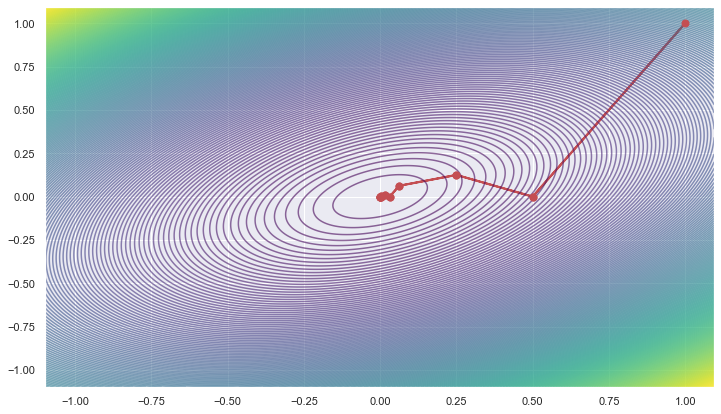
Conclusion
In this article, we familiarised ourselves with some of the useful techniques to optimize for the step size in the gradient descent algorithm. In particular, we covered 3 main techniques: Fixed Step Size, which involves maintaining the same step size or learning rate throughout the training process, Exact Line Search, which involves minimizing the loss as a function of t, and Armijo Backtracking involving a gradual reduction in the step size until a threshold is met. While these are some of the most fundamental techniques that you can use to tune your optimization, there exist a vast array of other methods (eg. setting t as a function of the number of iterations). These tools are generally used in more complex settings, such as Stochastic Gradient Descent. The purpose of this article was not only to introduce you to these techniques but also to make you aware of the intricacies that can affect your optimization algorithm. While most of these techniques are used in the context of Gradient descent, they can also be applied to other optimization algorithms (e.g., Newton-Raphson Method). Each of these techniques has its own merits and may be preferred over the others for specific applications and algorithms.
Hope you enjoyed reading this article! In case you have any doubts or suggestions, do reply in the comment box. Please feel free to contact me via mail.
If you liked my article and want to read more of them, please follow me.
Note: All images have been made by the author.
