Introducing Time Series in pandas

Quick Success Data Science

Data referenced to a time index is called a time series. Think of stock prices, temperature readings, and Google Trends. While I don't know anyone who likes working with time series, Python does its best to make it as easy as possible.

Python and its pandas data analysis library treat dates and times as special objects that are "aware" of the mechanics of the Gregorian calendar, the sexagesimal (base 60) time system, time zones, daylight-saving time, leap years, and more. Native Python supports times series through its [Datetime](https://docs.python.org/3/library/datetime.html) module, and pandas is oriented toward using arrays of dates, such as for an index or column in a DataFrame.

We'll review how pandas handles dates and times in this Quick Success Data Science article. The goal is to introduce you to the basics of working with time series in pandas and to make you conversant in the subject. For even more detail, you can visit the pandas user guide. If you need to install pandas, see the Getting Started guide.

---

Time Concepts in pandas

As you might expect, pandas has extensive capabilities for working with time series. This functionality is based on the NumPy datetime64 and timedelta64 data types with nanosecond resolution.

In addition, features have been consolidated from many other Python libraries and new functionality has been developed. With pandas, you can load time series; convert data to the proper datetime format; generate ranges of datetimes; index, merge, and resample both fixed- and irregular-frequency data; and more.

The pandas library uses four general time-related concepts. These are date times, time deltas, time spans, and date offsets. Except for date offsets, each time concept has a scalar class for single observations and an associated array class, which serves as an index structure.

A date time represents a specific date and time with time zone support. It's similar to datetime.datetime from the Python standard library.

A time delta is an absolute time duration, similar to datetime.timedelta from the standard library.

Time spans are periods defined by a point in time and its associated frequency (daily, monthly, and so on).

A date offset represents a relative time duration that respects calendar arithmetic.

In the sections that follow, we'll look at these various concepts and the methods used to create them. For more details, you can visit the official documentation.

---

Parsing Time Series Information

To create a timestamp representing the time for a particular event, use the Timestamp class (shown here in the Jupyter QT console):

In [1]: import pandas as pd

In [2]: ts = pd.Timestamp('2021-02-23 00:00:00')

In [3]: ts
Out[3]: Timestamp('2021-02-23 00:00:00')

Likewise, to create a DatetimeIndex object, use the DatetimeIndex class:

In [4]: dti = pd.DatetimeIndex(['2022-03-31 14:39:00', 
                        '2022-04-01 00:00:00'])

In [5]: dti
Out[5]: DatetimeIndex(['2022-03-31 14:39:00', '2022-04-01 00:00:00'], 
                      dtype='datetime64[ns]', freq=None)

For existing data, the [to_datetime()](https://pandas.pydata.org/pandas-docs/stable/reference/api/pandas.to_datetime.html) method converts scalar, array-like, dictionary-like, and pandas series or DataFrame objects to pandas datetime64[ns] objects. This lets you easily parse time series information from various sources and formats.

To see what I'm talking about, in a console or terminal, enter the following:

In [6]: import numpy as np
   ..:  from datetime import datetime
   ..:  import pandas as pd

In [7]: dti = pd.to_datetime(["2/23/2021",
                      np.datetime64("2021-02-23"),
                      datetime(2022, 2, 23)])

In [8]: dti
Out[8]: DatetimeIndex(['2021-02-23', '2021-02-23', '2022-02-23'], 
dtype='datetime64[ns]', freq=None)

In this example, we passed a list of dates in three different formats to the to_datetime() method. These included a string, a NumPy datetime64 object, and a Python datetime object. The method returned a pandas DatetimeIndex object that consistently stored the dates as datetime64[ns] objects in ISO 8601 format (year-month-day).

The method can accommodate times as well as dates:

 In [9]: dates = ['2022-3-31 14:39:00',
                 '2022-4-1 00:00:00',
                 '2022-4-2 00:00:20',
                 '']

In [10]: dti = pd.to_datetime(dates)

In [11]: dti
Out[11]: DatetimeIndex(['2022-03-31 14:39:00', '2022-04-01 00:00:00',
                        '2022-04-02 00:00:20', 'NaT'],
                       dtype='datetime64[ns]', freq=None)

In this example, we passed a list of both dates and times, which were all correctly converted. Note that we included an empty item at the end of the list. The to_datetime() method converted this entry into a NaT (Not a Time) value, which is the timestamp equivalent of the pandas NaN (Not a Number).

The to_datetime() method also works with pandas DataFrames. Let's look at an example in which you have recorded (in a spreadsheet like Excel) the date and time a trail camera captured an image of an animal. You've exported the spreadsheet as a .csv file that you now want to load and parse using pandas. To create the .csv file, in a text editor such as Notepad or TextEdit, enter the following and then save it as _camera1.csv:

Date,Obs
3/30/22 11:43 PM,deer
3/31/22 1:05 AM,fox
4/1/22 2:54 AM,cougar

Back in the console, enter the following to read the file in as a DataFrame (substitute your path to the .csv file):

In [12]: csv_df = pd.read_csv('C:/Users/hanna/camera_1.csv')

In [13]: csv_df
Out[13]: 
              Date  Obs
0 3/30/22 11:43 PM deer
1  3/31/22 1:05 AM fox
2   4/1/22 2:54 AM cougar

To convert the "Date" column to ISO 8601 format, enter the following:

In [14]: csv_df['Date'] = pd.to_datetime(csv_df['Date'])

In [15]: csv_df
Out[15]: 
                 Date  Obs
0 2022-03-30 23:43:00 deer
1 2022-03-31 01:05:00 fox
2 2022-04-01 02:54:00 cougar

These datetimes were recorded in the Eastern US time zone, but that information is not encoded. To make the datetimes aware, first make the following import:

In [16]: import pytz

Next, assign a variable to a pytz tzfile object and then pass the variable to the [tz_localize()](https://pandas.pydata.org/pandas-docs/stable/reference/api/pandas.Series.dt.tz_localize.html) method:

In [17]: my_tz = pytz.timezone('US/Eastern')

In [18]: csv_df['Date'] = csv_df['Date'].dt.tz_localize(my_tz)

You can do all this in one line but using a my_tz variable makes the code more readable and less likely to wrap. To check the results, print the "Date" column:

In [19]: print(csv_df['Date'])
0 2022-03-30 23:43:00-04:00
1 2022-03-31 01:05:00-04:00
2 2022-04-01 02:54:00-04:00
Name: Date, dtype: datetime64[ns, US/Eastern]

Even though it's a good idea to work in UTC, it's also important to have meaningful time data. For example, you'll probably want to study when these animals are on the prowl in local time, so you'll want to preserve the times recorded in the Eastern US.

In this case, you'll want to make a new "UTC-aware" column based on the "Date" column so that you can have the best of both worlds. Because the "Date" column is now aware of its time zone, you must use [tz_convert()](https://pandas.pydata.org/pandas-docs/stable/reference/api/pandas.Series.dt.tz_convert.html) instead of tz_localize():

In [20]: csv_df['Date_UTC'] = csv_df['Date'].dt.tz_convert(pytz.utc)

In [21]: print(csv_df[['Date', 'Date_UTC']])
                       Date                  Date_UTC
0 2022-03-30 23:43:00-04:00 2022-03-31 03:43:00+00:00
1 2022-03-31 01:05:00-04:00 2022-03-31 05:05:00+00:00
2 2022-04-01 02:54:00-04:00 2022-04-01 06:54:00+00:00

NOTE: To remove time zone information from a datetime so that it becomes naive, pass the tz_convert() method None, like so:

csv_df['Date'] = csv_df['Date'].dt.tz_ convert(None).

Finally, if you look at the previous printout of the csv_df DataFrame, you'll see that the index values range from 0 to 2. This is by default, but there's no reason why you can't use datetime values as the index instead. In fact, datetime indexes can be helpful when doing things like plotting. So, let's make the "Date_UTC" column the index for the DataFrame.

In a console, enter the following:

In [22]: csv_df = csv_df.set_index('Date_UTC')
Out[22]: 
                                         Date Obs
Date_UTC 
2022-03-31 03:43:00+00:00 2022-03-31 03:43:00 deer
2022-03-31 05:05:00+00:00 2022-03-31 05:05:00 fox
2022-04-01 06:54:00+00:00 2022-04-01 06:54:00 cougar

---

Creating Date Ranges

Time series with a fixed frequency occur often in science for jobs as diverse as sampling waveforms in signal processing, observing target behaviors in psychology, recording stock market movements in economics, and logging traffic flow in transportation engineering. Not surprisingly, pandas ships with standardized frequencies and tools that generate them, resample them, and infer them.

The pandas date_range() method returns a DatetimeIndex object with a fixed frequency. To generate an index composed of days, pass it a start and end date, as follows:

In [23]: day_index = pd.date_range(start='2/23/21', end='3/1/21')

In [24]: day_index
Out[24]: 
DatetimeIndex(['2021-02-23', '2021-02-24', '2021-02-25', '2021-02-26',
'2021-02-27', '2021-02-28', '2021-03-01'],
dtype='datetime64[ns]', freq='D')

You can also pass date_range() either a start date or an end date, along with the number of periods to generate. In the following example, we start with a timestamp for a certain observation and ask for six periods:

In [25]: day_index = pd.date_range(start='2/23/21 12:59:59', periods=6)

In [26]: day_index
Out[26]: 
DatetimeIndex(['2021-02-23 12:59:59', '2021-02-24 12:59:59',
'2021-02-25 12:59:59', '2021-02-26 12:59:59',
'2021-02-27 12:59:59', '2021-02-28 12:59:59'],
dtype='datetime64[ns]', freq='D')

Note that the six datetimes represent days starting at 12:59:59. Normally, you want the days to start at midnight, so, pandas provides a handy normalize parameter to make this adjustment:

In [27]: day_index_normal = pd.date_range(start='2/23/21 12:59:59',
     ..:                                  periods=6, 
     ..:                                  normalize=True)

In [28]: day_index_normal
Out[28]: 
DatetimeIndex(['2021-02-23', '2021-02-24', '2021-02-25', '2021-02-26',
'2021-02-27', '2021-02-28'],
dtype='datetime64[ns]', freq='D')

After they're normalized to days, the output datetime64 objects no longer include a time component.

By default, the date_range() method assumes that you want a daily frequency. Other frequencies are available, however, with many designed for business applications (such as the end of a business month, end of a business year, and so on).

The following table lists some of the time series frequencies more relevant for science. For the complete list, including financial frequencies, see "DateOffset objects" here.

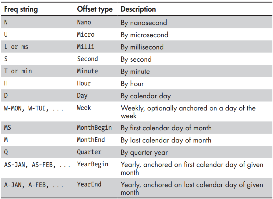
To specify an offset type, pass a frequency string alias from the previous table as the freq argument. You can also specify a time zone using the tz argument. Here's how to make an hourly frequency referenced to UTC:

In [29]: hour_index = pd.date_range(start='2/23/21', 
     ..:                            periods=6, 
     ..:                            freq='H', 
     ..:                            tz='UTC')

In [30]: hour_index
Out[30]: 
DatetimeIndex(['2021-02-23 00:00:00+00:00', '2021-02-23 01:00:00+00:00',
'2021-02-23 02:00:00+00:00', '2021-02-23 03:00:00+00:00',
'2021-02-23 04:00:00+00:00', '2021-02-23 05:00:00+00:00'],
dtype='datetime64[ns, UTC]', freq='H')

For an existing time series, you can retrieve its frequency by using the freq attribute, as shown here:

In [31]: hour_index.freq
Out[31]: 

The frequencies shown in the previous table represent base frequencies. Think of these as building blocks for alternative frequencies, such as bi-hourly. To make this new frequency, just place the integer 2 before the H in the freq argument, as follows:

In [32]: bi_hour_index = pd.date_range(start='2/23/21', periods=6, freq='2H')

In [33]: bi_hour_index
Out[33]: 
DatetimeIndex(['2021-02-23 00:00:00', '2021-02-23 02:00:00',
'2021-02-23 04:00:00', '2021-02-23 06:00:00',
'2021-02-23 08:00:00', '2021-02-23 10:00:00'],
dtype='datetime64[ns]', freq='2H')

You can also combine offsets by passing frequency strings like ‘2H30min', like this:

In [34]: pd.date_range(start='2/23/21', periods=6, freq='2H30min')
Out[34]:
DatetimeIndex(['2021-02-23 00:00:00', '2021-02-23 02:30:00',
'2021-02-23 05:00:00', '2021-02-23 07:30:00',
'2021-02-23 10:00:00', '2021-02-23 12:30:00'],
dtype='datetime64[ns]', freq='150T')

---

Creating Periods

Timestamps associate data with points in time. Sometimes, however, data remains constant through a certain time span, such as a month, and you want to associate the data with that interval.

In pandas, regular intervals of time such as a day, month, year, and so on are represented by [Period](https://pandas.pydata.org/docs/reference/api/pandas.Period.html) objects. With the period_range() method, Period objects can be collected into a sequence to form a PeriodIndex. You can specify a period's time span using the freq keyword with frequency aliases from the previous table.

Suppose you want to keep track of a daily observation for September 2022. First, use the period_range() method to create a period with a frequency of days:

In [35]: p_index = pd.period_range(start='2022-9-1', 
     ..:                           end='2022-9-30', 
     ..:                           freq='D')

Next, create a pandas series and use the NumPy random.randn() method to generate some fake data on the fly. Note that the number of data points must equal the number of days in the index:

In [36]: ts = pd.Series(np.random.randn(30), index=p_index)

In [37]: ts
Out[37]: 
2022-09-01 0.412853
2022-09-02 0.350678
2022-09-03 0.086216

--snip--

2022-09-28 1.944123
2022-09-29 0.311337
2022-09-30 0.906780
Freq: D, dtype: float64

You now have a time series, organized by day, for the month of September.

To shift a period by its own frequency, just add or subtract an integer. Here's an example using a yearly time span:

In [38]: year_index = pd.period_range(2001, 2006, freq='A-DEC')

In [39]: year_index
Out[39]: PeriodIndex(['2001', '2002', '2003', '2004', '2005', '2006'], 
dtype='period[A-DEC]')

In [40]: year_index + 10
Out[40]: PeriodIndex(['2011', '2012', '2013', '2014', '2015', '2016'], 
dtype='period[A-DEC]')

Using a frequency of A-DEC means that each year represents January 1 through December 31. Adding 10 shifted the periods up by 10 years. You can only perform arithmetic in this manner between Period objects with the same frequency.

Here's an example of making monthly periods:

In [41]: month_index = pd.period_range('2022-01-01', '2022-12-31', freq='M')

In [42]: month_index
Out[42]: 
PeriodIndex(['2022-01', '2022-02', '2022-03', '2022-04', '2022-05', '2022-06', 
'2022-07', '2022-08', '2022-09', '2022-10', '2022-11', '2022-12'],
dtype='period[M]')

With the [asfreq()](https://pandas.pydata.org/docs/reference/api/pandas.Period.asfreq.html) method, you can convert an existing period to another frequency. Here's an example in which we convert the month_index variable's period to hours, anchored on the first hour of each month:

In [43]: hour_index = month_index.asfreq('H', how='start')

In [44]: hour_index
Out[44]: 
PeriodIndex(['2022-01-01 00:00', '2022-02-01 00:00', '2022-03-01 00:00',
'2022-04-01 00:00', '2022-05-01 00:00', '2022-06-01 00:00',
'2022-07-01 00:00', '2022-08-01 00:00', '2022-09-01 00:00',
'2022-10-01 00:00', '2022-11-01 00:00', '2022-12-01 00:00'],
dtype='period[H]')

---

Creating Time Deltas

The timedelta_range() method creates TimedeltaIndex objects. It behaves similarly to date_range() and period_range():

In [45]: pd.timedelta_range(start='1 day', periods = 5)
Out[45]: TimedeltaIndex(['1 days', '2 days', '3 days', '4 days', '5 days'], 
dtype='timedelta64[ns]', freq='D')

In the television drama Lost, a character had to enter a code and push a button every 108 minutes to avert some unknown catastrophe. With the timedelta_range() method and a frequency argument, he could schedule his day around this requirement. Assuming he last pushed the button at midnight, he won't be getting much uninterrupted sleep:

In [46]: pd.timedelta_range(start="1 day", end="2 day", freq="108min")
Out[46]: 
TimedeltaIndex(['1 days 00:00:00', '1 days 01:48:00', '1 days 03:36:00',
'1 days 05:24:00', '1 days 07:12:00', '1 days 09:00:00',
'1 days 10:48:00', '1 days 12:36:00', '1 days 14:24:00',
'1 days 16:12:00', '1 days 18:00:00', '1 days 19:48:00',
'1 days 21:36:00', '1 days 23:24:00'],
dtype='timedelta64[ns]', freq='108T')

---

Shifting Dates with Offsets

In addition to working with frequencies, you can import offsets and use them to shift Timestamp and DatetimeIndex objects. Here's an example in which we import the Day class and use it to shift a famous date:

In [47]: from pandas.tseries.offsets import Day

In [48]: apollo_11_moon_landing = pd.to_datetime('1969, 7, 20')

In [49]: apollo_11_splashdown = apollo_11_moon_landing + 4 * Day()

In [50]: print(f"{apollo_11_splashdown.month}/{apollo_11_splashdown.day}")
7/24

You can also import DateOffset class and then pass it the time span as an argument:

In [51]: from pandas.tseries.offsets import DateOffset

In [52]: ts = pd.Timestamp('2021-02-23 09:10:11')

In [53]: ts + DateOffset(months=4)
Out[53]: Timestamp('2021-06-23 09:10:11')

A nice thing about DateOffset objects is that they honor DST transitions. You just need to import the appropriate class from pandas.tseries.offsets. Here's an example of shifting one hour across the vernal DST transition in the US Central time zone:

In [54]: from pandas.tseries.offsets import Hour

In [55]: pre_dst_date = pd.Timestamp('2022-03-13 1:00:00', tz='US/Central')

In [56]: pre_dst_date
Out[56]: Timestamp('2022-03-13 01:00:00-0600', tz='US/Central')

In [57]: post_dst_date = pre_dst_date + Hour()

In [58]: post_dst_date
Out[58]: Timestamp('2022-03-13 03:00:00-0500', tz='US/Central')

Note that the final datetime (03:00:00) is two hours later than the starting datetime (01:00:00), even though you shifted it one hour. This is due to crossing the DST transition.

Along these lines, you can combine two time series even if they are in different time zones. The result will be in UTC, as pandas automatically keeps track of the equivalent UTC timestamps for each time series. To see the long list of available offsets, visit the docs.

---

Indexing and Slicing Time Series

When you're working with time series data, it's conventional to use the time component as the index of a series or DataFrame so that you can perform manipulations with respect to the time element. Here, we make a series whose index represents a time series and whose data is the integers 0 through 9:

In [59]: ts = pd.Series(range(10), index=pd.date_range('2022', 
     ..:                                               freq='D', 
     ..:                                               periods=10))

In [60]: ts
Out[60]: 
2022-01-01 0
2022-01-02 1
2022-01-03 2
2022-01-04 3
2022-01-05 4
2022-01-06 5
2022-01-07 6
2022-01-08 7
2022-01-09 8
2022-01-10 9
Freq: D, dtype: int64

Even though the indexes are now dates, you can slice and dice the series, just as with integer indexes. For example, to select every other row, enter the following:

In [61]: ts[::2]
Out[61]: 
2022-01-01 0
2022-01-03 2
2022-01-05 4
2022-01-07 6
2022-01-09 8
Freq: 2D, dtype: int64

To select the data associated with the January 5, index the series using that date:

In [62]: ts['2022-01-05']
Out[62]: 4

Conveniently, you don't need to enter the date in the same format that it was input. Any string interpretable as a date will do:

In [63]: ts['1/5/2022']
Out[63]: 4

In [64]: ts['January 5, 2022']
Out[64]: 4

Duplicate dates will produce a slice of the series showing all values associated with that date. Likewise, you will see all the rows in a DataFrame indexed by the same date using the syntax: dataframe.loc[_'datetimeindex'].

Additionally, if you have a time series with multiple years, you can index based on the year and retrieve all the indexes and data that include that year. This also works for other timespans, such as months. Slicing works the same way. You can use timestamps not explicitly included in the time series, such as 2021–12–31:

In [65]: ts['2021-12-31':'2022-1-2']
Out[65]: 
2022-01-01 0
2022-01-02 1
Freq: D, dtype: int64

In this case, we started indexing with December 31, 2021, which precedes the dates in the time series.

NOTE: Remember that pandas is based on NumPy, so slicing creates views rather than copies. Any operation you perform on a view will change the source series or DataFrame.

If you want the datetime component to be the data instead of the index, leave off the index argument when creating the series:

In [66]: pd.Series(pd.date_range('2022', freq='D', periods=3))
Out[66]: 
0 2022-01-01
1 2022-01-02
2 2022-01-03
dtype: datetime64[ns]

The result is a pandas series with an integer index and the dates treated as data.

---

Resampling Time Series

The process of converting the frequency of a time series to a different frequency is called resampling. This can involve downsampling, by which you aggregate data to a lower frequency, perhaps to reduce memory requirements or see trends in the data; upsampling, wherein you move to a higher frequency, perhaps to permit mathematical operations between two datasets with different resolutions; or simple resampling, for which you keep the same frequency but change the anchor point from, say, the start of the year (AS-JAN) to the year-end (A-JAN).

In pandas, resampling is accomplished by calling the resample() method on a pandas object using dot notation. Some of its commonly used parameters are listed in the following table. To see the complete list, visit the docs. Both series and dataframe objects use the same parameters.

---

Upsampling

Upsampling refers to resampling to a shorter time span, such as from daily to hourly. This creates bins with NaN values that must be filled; for example, as with the forward-fill and backfill methods ffill() and bfill(). This two-step process can be accomplished by chaining together the calls to the resample and fill methods.

To illustrate, let's make a toy dataset with yearly values and expand it to quarterly values. This might be necessary when, say, production targets go up every year, but progress must be tracked against quarterly production. In the console, enter the following:

In [67]: import pandas as pd

In [68]: dti = pd.period_range('2021-02-23', freq='Y', periods=3)

In [69]: df = pd.DataFrame({'value': [10, 20, 30]}, index=dti)

In [70]: df.resample('Q').ffill()

After importing pandas, establish an annual PeriodIndex named dti. Next, create the DataFrame and pass it a dictionary with the values in list form. Then, set the index argument to the dti object. Call the resample() method and pass it Q, for quarterly, and then call the ffill() method, chained to the end.

The results of this code are broken down in the next figure, which, from left to right, shows the original DataFrame, the resampling results, and the fill results. The original annual values are shown in bold.

The resample() method builds the new quarterly index and fills the new rows with NaN values. Calling ffill() fills the empty rows going "forward." What you're saying here is, "The value for the first quarter of each year (Q1) is the value to use for all quarters within that year."

Backfilling does the opposite and assumes that the value at the start of each new year (Q1) should apply to the quarters in the previous year excluding the previous first quarter:

In [71]: df.resample('Q').bfill()

The execution of this code is described by the following figure. Again, original annual values are shown in bold.

In this case, the values associated with the first quarter are "backfilled" to the previous three quarters. You must be careful, however, as "leftover" NaNs can occur. You can see these at the end of the value column in the right-hand DataFrame in the previous figure. The last three values are unchanged because no 2024Q1 data was available to set the value.

To fill the missing data, let's assume that the values keep increasing by 10 each quarter and rerun the code using the fillna() method chained to the end. Pass it 40 to fill the remaining holes:

In [72]: df.resample('Q').bfill().fillna(40)
Out[72]: 
      value
2021Q1 10.0
2021Q2 20.0
2021Q3 20.0
2021Q4 20.0
2022Q1 20.0
2022Q2 30.0
2022Q3 30.0
2022Q4 30.0
2023Q1 30.0
2023Q2 40.0
2023Q3 40.0
2023Q4 40.0

Both bfill() and ffill() are synonyms for the fillna() method. You can read more about it here.

---

Downsampling

Downsampling refers to resampling from a higher frequency to a lower frequency, such as from minutes to hours. Because multiple samples must be combined into one, the resample() method is usually chained to a method for aggregating the data:

To practice downsampling, we'll use a real-world dataset from "The COVID Tracking Project" at The Atlantic. This dataset includes COVID-19 statistics from March 3, 2020, to March 7, 2021. To reduce the size of the dataset, we'll use the data for just the state of Texas.

If you want to download this data and follow along, navigate to this page, scroll down, and then click the link for Texas. The license for the data is here

The following code loads the data as a pandas DataFrame. The input file has many columns of data that we don't need, so select only the "date" and "deathIncrease" columns. The latter column is the number of COVID-related deaths for the day.

In [73]: df = pd.read_csv("texas-history.csv", 
    ...: usecols=['date','deathIncrease'])

In [74]: df.head()
Out[74]: 
         date deathIncrease
0 2021-03-07             84
1 2021-03-06            233
2 2021-03-05            256
3 2021-03-04            315
4 2021-03-03            297

It's good to keep an eye on what's happening to the data by calling the head() method on the DataFrame, which returns the first five rows by default. Here, we see that dates are organized in descending order, but we generally use and plot datetime data in ascending order. So, call the pandas sort_values() method, pass it the column name, and set the ascending argument to True:

In [75]: df = df.sort_values('date', ascending=True)
In [76]: df.head()
Out[76]: 
          date deathIncrease
369 2020-03-03             0
368 2020-03-04             0
367 2020-03-05             0
366 2020-03-06             0
365 2020-03-07             0

Next, the dates look like dates, but are they? Check the DataFrame's dtypes attribute to confirm one way or the other:

In [77]: df.dtypes
Out[77]: 
date object
deathIncrease int64
dtype: object

They're not. This is important because the resample() method works only with objects having a datetime-like index, such as DatetimeIndex, PeriodIndex, or TimedeltaIndex. We'll need to change their type and set them as the DataFrame's index, replacing the current integer values. We'll also drop the date column because we no longer need it:

In [78]: df = df.set_index(pd.DatetimeIndex(df['date'])).drop('date',
    ...:                                                      axis=1)

In [79]: df.head()
Out[79]: 
           deathIncrease
date 
2020-03-03             0
2020-03-04             0
2020-03-05             0
2020-03-06             0
2020-03-07             0

At this point, we've wrangled the data so that our DataFrame uses a DatetimeIndex with dates in ascending order. Let's see how it looks by making a quick plot using pandas plotting, which is quick and easy for data exploration:

In [80]: df.plot();

One aspect of this figure that stands out is the spike in values near the start of August 2020. Because this is a maximum value, you can easily retrieve the value and its date index by using the max() and idxmax() methods, respectively:

In [81]: print(df.max(), df.idxmax())
deathIncrease 675
dtype: int64 deathIncrease 2020-07-27
dtype: datetime64[ns]

This value is likely incorrect, given that the CDC records only 239 deaths on this date, which is more consistent with the adjacent data. Let's use the CDC value going forward. To change the DataFrame, we can apply the .loc indexer, passing it the date (index) and column name, as follows:

In [82]: df.loc['2020-7-27', 'deathIncrease'] = 239

In [83]: df.plot();

The spike is gone now, and the plot looks more reasonable, as demonstrated below:

Another noticeable thing is the "sawtooth" nature of the curve caused by periodic oscillations in the number of deaths. These oscillations have a high frequency, and it's doubtful that the disease progressed this way.

To investigate this anomaly, we'll make a new DataFrame that includes a column for weekdays:

In [84]: df_weekdays = df.copy()

In [85]: df_weekdays['weekdays'] = df.index.day_name()

Now, let's print out multiple weeks' worth of data using pandas' iloc[] indexing:

In [86]: print(df_weekdays.iloc[90:115])

As I've highlighted in gray, the lowest reported number of deaths consistently occurs on a Monday, and the Sunday results also appear suppressed. This suggests a reporting issue over the weekend, with a one-day time lag. You can read more about this reporting phenomenon here.

Because the oscillations occur weekly, downsampling from daily to weekly should merge the low and high reports and smooth the curve. Let's test the hypothesis:

In [87]: df.resample('W').sum().plot();

The high-frequency oscillations are gone.

Now, let's downsample to a monthly period:

In [88]: df.resample('m').sum().plot();

This produced an even smoother plot. Note that you can also downsample to custom periods, such as ‘4D', for every four days.

---

Changing the Start Date When Resampling

So far, we've been taking the default origin (start date) when aggregating intervals, but this can lead to unwanted results. Here's an example:

In [89]: raw_dict = {'2022-02-23 09:00:00': 100,
    ...:             '2022-02-23 10:00:00': 200,
    ...:             '2022-02-23 11:00:00': 100,
    ...:             '2022-02-23 12:00:00': 300}

In [90]: ts = pd.Series(raw_dict)

In [91]: ts.index = pd.to_datetime(ts.index)

In [92]: ts.resample('2H').sum()
Out[92]: 
2022-02-23 08:00:00 100
2022-02-23 10:00:00 300
2022-02-23 12:00:00 300
Freq: 2H, dtype: int64

Despite the first data point being recorded at 9 AM, the resampled sums start at 8 AM. This is because the default for aggregated intervals is 0, causing the two-hour ('2H') frequency timestamps to be 00:00:00, . . . 08:00:00, 10:00:00, and so on, skipping 09:00:00.

To force the output range to start at 09:00:00, pass 'start'to the method's origin argument. Now it should use the actual start of the time series:

In [93]: ts.resample('2H', origin='start').sum()
Out[93]: 
2022-02-23 09:00:00 300
2022-02-23 11:00:00 400
Freq: 2H, dtype: int64

The aggregation now starts at 9 AM, as desired.

---

Resampling Irregular Time Series Using Interpolation

Scientific observations are often irregular in nature. After all, wildebeests don't show up at waterholes on a fixed schedule. Fortunately, resampling works the same whether a time series has an irregular or fixed frequency.

As with upsampling, regularizing a time series will generate new timestamps with empty values. Previously, we filled these blank values using backfilling and front-filling. In the next example, we'll use the pandas [interpolate()](https://pandas.pydata.org/pandas-docs/stable/reference/api/pandas.Series.interpolate.html) method.

Let's begin by generating a list of irregularly spaced datetimes with a resolution measured in seconds:

In [94]: raw = ['2021-02-23 09:46:48',
     ...:       '2021-02-23 09:46:51',
     ...:       '2021-02-23 09:46:53',
     ...:       '2021-02-23 09:46:55',
     ...:       '2021-02-23 09:47:00']

Next, in a single line, we create a pandas series object where the index is the datetime string converted to a DatetimeIndex:

In [95]: ts = pd.Series(np.arange(5), index=pd.to_datetime(raw))

In [96]: ts
Out[96]: 
2021-02-23 09:46:48 0
2021-02-23 09:46:51 1
2021-02-23 09:46:53 2
2021-02-23 09:46:55 3
2021-02-23 09:47:00 4
dtype: int32

Now, we resample this time series at the same resolution ('s') and call interpolate() using 'linear' for the method argument:

In [97]: ts_regular = ts.resample('s').interpolate(method='linear')

In [98]: ts_regular
Out[98]: 
2021-02-23 09:46:48 0.000000
2021-02-23 09:46:49 0.333333
2021-02-23 09:46:50 0.666667
2021-02-23 09:46:51 1.000000
2021-02-23 09:46:52 1.500000
2021-02-23 09:46:53 2.000000
2021-02-23 09:46:54 2.500000
2021-02-23 09:46:55 3.000000
2021-02-23 09:46:56 3.200000
2021-02-23 09:46:57 3.400000
2021-02-23 09:46:58 3.600000
2021-02-23 09:46:59 3.800000
2021-02-23 09:47:00 4.000000
Freq: S, dtype: float64

We now have timestamps for every second, and new values have been interpolated between the original data points. The method argument comes with other options, including nearest, pad, zero, spline, and more.

Resampling and Analyzing Irregular Time Series: A Binary Example

Let's look at a realistic example of working with irregular time series. Imagine that you've attached a sensor to the compressor of a refrigeration unit to see how often it's on (1) and off (0) during a day.

To build the toy dataset, enter the following in the console:

In [99]: raw_dict = {'2021-2-23, 06:00:00': 0,
    ...:             '2021-2-23, 08:05:09': 1,
    ...:             '2021-2-23, 08:49:13': 0,
    ...:             '2021-2-23, 11:23:21': 1,
    ...:             '2021-2-23, 11:28:14': 0}

In [100]: ts = pd.Series(raw_dict)

In [101]: ts.index = pd.to_datetime(ts.index)

In [102]: ts.plot();

This produces the following plot. Note that it doesn't reflect the data's binary (0 or 1) nature.

In its raw, irregular form, the data is difficult to visualize and work with. For example, if you try to check the state of the compressor at 11 AM, you'll get an error:

In [103]: ts['2021-02-23 11:00:00']
KeyError --snip--

The problem is that series indexing doesn't interpolate on the fly. We need to first resample the data to a "working resolution," in this case, seconds:

In [104]: ts_secs = ts.resample('S').ffill()

In [105]: ts_secs
Out[105]:
2021-02-23 06:00:00 0
2021-02-23 06:00:01 0
2021-02-23 06:00:02 0
2021-02-23 06:00:03 0
2021-02-23 06:00:04 0
..
2021-02-23 11:28:10 1
2021-02-23 11:28:11 1
2021-02-23 11:28:12 1
2021-02-23 11:28:13 1
2021-02-23 11:28:14 0
Freq: S, Length: 19695, dtype: int64

In [106]: ts_secs.plot();

Now the plot reflects the binary "on-off" nature of the data, and you can extract the state at 11 AM:

In [107]: ts_secs['2021-2-23 11:00:00']
Out[107]: 0

To determine how many seconds the compressor was off and on during the time period, call the value_counts() method on the series:

In [108]: ts_secs.value_counts()
Out[108]: 
0 16758
1 2937
dtype: int64

To determine the fraction of the day that the compressor was on, just divide the value_counts() output at index 1 by the number of seconds in a day:

In [109]: num_secs_per_day = 60 * 60 * 24

In [110]: print(f"On = {ts_secs.value_counts()[1] / num_secs_per_day}")
On = 0.033993055555555554

The compressor ran for only three percent of the day. That's some good insulation!

---

Sliding Window Functions

The pandas library includes functions for transforming time series using a sliding window or exponentially decaying weights. These functions smooth raw data points so that long-term trends are more apparent.

A moving average is a commonly used time series technique for smoothing noise and gaps and revealing underlying data trends. Well-known examples are the 50- and 200-day moving averages used to analyze stock market data.

To make a moving average, rows in a DataFrame column are averaged using a "window" of a specified length. This window starts at the earliest date and slides down the column one time unit at a time, then repeats the process. Here's an example for a three-day moving average, with the averaged values in bold:

      date  value 
2020-06-01      6 |
2020-06-02     20 | |
2020-06-03     36 | | |--> (6 + 20 + 36)/3 = 20.67
2020-06-04     33 | |--> (20 + 36 + 33)/3 = 29.67
2020-06-05     21 |--> (36 + 33 + 21)/3 = 30.0

To make a "monthly" 30-day moving average of our COVID data from the earlier "Downsampling" section, we first reimport it as a new DataFrame named df_roll and replace the anomalous (spikey) value. (If you still have the data in memory, you can use df_roll = df.copy() in place of the next five lines):

In [111]: df_roll = pd.read_csv("texas-history.csv",
     ...:                       usecols = ['date','deathIncrease'])

In [112]: df_roll = df_roll.sort_values('date', ascending=True)

In [113]: df_roll = df_roll.set_index(pd.DatetimeIndex(df_roll['date']))

In [114]: df_roll = df_roll.drop('date', axis=1)

In [115]: df_roll.loc['2020-7-27', 'deathIncrease'] = 239

Next, we make a "30_day_ma" column for this DataFrame and calculate the values by calling the rolling() method on the "deathIncrease" column, passing it 30 and then tacking on the mean() method. We finish by calling plot():

In [116]: df_roll['30_day_ma'] = df_roll.deathIncrease.rolling(30).mean()

In [117]: df_roll.plot();

By default, the averaged values are posted at the end of the window, making the average curve look offset relative to the daily data. To post at the center of the window, pass True to the rolling() method's center argument:

In [118]: df_roll['30_day_ma'] = df_roll.deathIncrease.rolling(30,
      ..:                                                   center=True).mean()

In [119]: df_roll.plot();

Now, the peaks and valleys in the averaged curve and the raw data are better aligned:

You can call other aggregation methods with rolling(). Here, we call the standard deviation method on the same 30-day sliding window and display the new column with the others:

In [120]: df_roll['30_std'] = df_roll.deathIncrease.rolling(30,
      ..:                                                   center=True).std()

In [121]: df_roll.plot();

In addition to rolling averages with a fixed-sized window, pandas has methods for using expanding windows (expanding()), binary moving windows (corr()), exponentially weighted functions (ewm()), and user-defined moving window functions (apply()).

---

The Recap

Time series represent data indexed chronologically. Pandas provides special "time-aware" data types and tools for working with time series. These let you easily handle issues like sexagesimal arithmetic, time zone transitions, daylight saving time, leap years, datetime plotting, and more.

For a similar introduction to Python's datetime module, see my article:

Introducing Python's datetime Module

---

Thanks!

Thanks for reading. This article represents an extract from my latest book, Python Tools for Scientists. If you found it useful, please check out the book online or in a nearby bookstore. And be sure to follow me for more Quick Success Data Science articles in the future.

Python Tools for Scientists: An Introduction to Using Anaconda, JupyterLab, and Python's Scientific…

Tags: Datetime Deep Dives Pandas Tutorial Python Programming Time Series Analysis

Comment