Introduction to Reinforcement Learning and Solving the Multi-armed Bandit Problem
Reinforcement Learning (RL) is a fascinating subfield of Machine Learning. You might already know it from applications such as playing Go [1], autonomous driving [2], and more.
Equally fascinating in my opinion is Sutton's and Barto's famous book, "Reinforcement Learning" [3]. I think it's a great introduction to the topic, but also dives deep and introduces all important theoretical topics of the field. It can be a lot to read though, and especially upon the first read might look a bit mathy.

Thus, I decided to start a post series summarizing the book chapter by chapter. I believe getting the contents explained with different words will greatly help understanding. And I will also implement all (most) algorithms from the book in Python and apply them to problems and environments modeled via (formerly) OpenAI's gymnasium framework [4]. These two points are, as far as I know, novel so far and make this series unique.
This post is the first in the series, and will briefly introduce RL in general, then give a quick overview of how Sutton's book is structured – and how we will cover it. The main part of this post is then Chapter II of Sutton's book, which introduces RL in a nonassociative setting – using multi-armed bandits.
Short Introduction to Reinforcement Learning
RL, as opposed to e.g. supervised learning, does not learn from a fixed dataset of labelled examples, but instead learns by interacting with an environment and aiming to maximize a pre-defined reward function. We'll formalize this in more detail in the next post using Markov decision processes, but, briefly speaking: we have an agent, who acts within an environment. In every state the agent is in, it can take an action, observe the reward obtained due to taking said action in this state, and move to the next state. We can then apply a multitude of methods (such as Q-Learning, PPO …) for solving this problem and obtaining a policy: a mapping from states to actions, describing how the agent is supposed to behave in every state. As we can see, RL is a seemingly simple formulation and solution procedure, but of course comes with difficulties too: it is crucial to specify good rewards, and not immediately clear what the best choice for this is – and also the process of solving the problem comes with challenges such as instabilities and high variance.
Overview of "Reinforcement Learning" by Sutton and Barto
In this section we'll briefly sketch the contents of Sutton's book – in the process simultaneously also giving an outlook of posts to come in this series. While doing so we'll use the second edition, which is freely available under this link.
The book is split into three parts: in Part 1, tabular solution methods are discussed. This means, the state and action spaces are small enough s.t. we can represent the whole problem and also the found policy as a table – describing which action to take in which state. For this, given enough compute, we can usually find the optimal solution. Three general solution methods are presented: Dynamic Programming (DP), Monte Carlo Methods (MC), and Temporal-Difference Learning (TD) – all with their own strengths and weaknesses. DP is a general solving technique in computer science, in which solutions are built iteratively using recursion. In RL, they require a perfect model of the world since knowledge about future states is needed – but for that they are well understood and more easily analyzed. MC methods do not require a model, and instead roll out full episodes while observing returns. They are conceptually simpler, but cannot be used for iterative algorithms. Finally, TD methods combine both previous approaches: they do not need a model but directly learn from experience, and also bootstrap on previous solutions in iterative fashion. However, they are more complex to analyze.
In Part 2, we extend this to larger and more realistic problems: now, the problems / state and action spaces are assumed to be too large (or even infinite) to feasibly represent them in tabular fashion. That means we need to approximate and also accept finding less-than optimal solutions. The chapter starts by introducing function approximation: we need ways of parametrizing large input spaces, and learning just from a subset of all possible inputs. It then moves towards solving RL problems with approximation – which comes with several new challenges (one for example being the "deadly triad" of using function approximation, bootstrapping and off-policy training simultaneously). We also learn about alternatives to the classical state / action parametrization used everywhere until now – and get introduced to policy methods, which directly aim to learn a policy, and not state / action functions describing the "goodness" of states and actions.
Part 3 is an interesting extension beyond introductory principles – although I have to say I did not read all parts of this section very carefully. The chapter starts by linking RL to Psychology and Neuroscience, motivating RL algorithms from a biological perspective. Next, successful real-world RL applications are presented. Although some seem a bit old and outdated, there are also more recent, ground-breaking results such as playing Atari games or Go using RL. The chapter (and book) ends with a discussion about latest trends and frontiers of the field.
Multi-armed Bandits
With that, let's dive into Chapter 2 of Sutton's book and solve our first RL problem. The problem will involve multi-armed bandits, and takes place in a nonassociative setting – meaning there is only a single state and we have to find globally optimal best actions – as opposed to the more standard associative setting, in which one has to find best actions for different states.
Multi-armed bandits are typical gambling machines, but often used to motivate problems involving statistics, RL, and more. This chapter might feel somewhat detached from "typical" RL problems – and in fact, it is. The setting is conceptually different from all the problems we will be solving in the next chapters. However, due to the aforementioned reason, multi-armed bandits are a good playing ground to slowly dive into this field: we will come into contact with many techniques and terms we will re-use later on, such as ε-greedy, value functions, policies, and co.
The setting is the following: imagine we find ourselves in a room with N (multi-armed) bandits, and are tasked to maximize our returns when playing these for a fixed amount of time. Each bandit only allows one action, namely pulling the designated lever / arm. When doing so, we obtain a specific reward, which follows a Gaussian distribution with a fixed mean / variance. If there was no randomness involved, one would simply try every machine once, and then continue playing the best bandit. However, since we do not have access to the true reward distribution, we face an exploration vs exploitation dilemma.
This is a common theme in RL: at every timestep we can be greedy, and exploit knowledge we have collected so far – such as playing that machine which empirically – up to now – yielded the most returns. However, this comes at the risk of missing out on other, potentially even better machines we discovered less so far. Therefore, it can be beneficial to explore more of the environment.
All methods of Part I of Sutton's book have in common that they explicitly compute and store values of states and actions, namely the state-value function v(s) and the action-value function q(s, a). Intuitively these describe the "goodness" of a certain state (v), or the "goodness" of taking action a in state s (q). If we have found these values, it is easy to define a policy yielding optimal returns: in each state, simply take the action corresponding to the highest q value. That might make sense intuitively – and in a later episode we will also formally show why such a greedy approach indeed yields the optimal result (hint: Bellman equation).
However, for the multi-armed bandit problem this notation simplifies somewhat due to the aforementioned nonassociative setting, and we only need an action-value function Q(a), with the optimal solution being:

That is, the optimal value of taking action a (which denotes playing the bandit corresponding to this index) should equal the expected return from the underlying reward distribution.
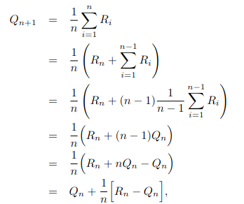
It seems nearby to estimate these values using the sample means, i.e. averaging historic means:

However, for this naive computation we would need to hold all previous results in memory – and using some simple reformulation we can reduce this to O(1) memory and an iterative formula:
Such an update pattern is very common in RL, with the general form being:

In fact, StepSize = 1/n assigns uniform weight to all observed rewards – which makes sense for multi-armed bandits, as rewards do not change over time. However, some analyzed problems are non-stationary, and also in general it makes more sense to weigh recent results higher. We can do so by setting StepSize equal to some constant alpha – which is a more common update rule.
Implementation
The above update procedure translates to an algorithm in straightforward fashion:

We use two variables, Q and N, to save estimated state values and action execution frequencies. We then continuously increment the value estimates, following an ε-greedy policy: with probability 1 – ε we exploit the current best action, with probability ε we explore a random action.
A particular focus of this series is to present executable Python code, so let's do exactly that. You can find the complete code on Github (if you are curious about some of the "design choices" in the repo, and how I organize my code – I may refer to a previous post). The core part is defining the ε-greedy policy (the criterion for choosing actions), as well as the solving algorithm bandit_solver representing above pseudocode:
from typing import Callable

import matplotlib.pyplot as plt
import numpy as np

NUM_STEPS = 1000

class Bandit:
    def __init__(self, mu: float, sigma: float = 1) -> None:
        self.mu = mu
        self.sigma = sigma

    def __call__(self) -> np.ndarray:
        return np.random.normal(self.mu, self.sigma, 1)

def initialize_bandits() -> list[Bandit]:
    return [
        Bandit(0.2),
        Bandit(-0.8),
        Bandit(1.5),
        Bandit(0.4),
        Bandit(1.1),
        Bandit(-1.5),
        Bandit(-0.1),
        Bandit(1),
        Bandit(0.7),
        Bandit(-0.5),
    ]

def simple_crit(Q: np.ndarray, N: np.ndarray, t: int, eps: float) -> int:
    return (
        int(np.argmax(Q))
        if np.random.rand() < 1 - eps
        else np.random.randint(Q.shape[0])
    )

def bandit_solver(
    bandits: list[Bandit], crit: Callable[[np.ndarray, np.ndarray, int], int]
) -> np.ndarray:
    Q = np.zeros((len(bandits)))
    N = np.zeros((len(bandits)))

    rewards = []
    for t in range(NUM_STEPS):
        A = crit(Q, N, t)
        R = bandits[A]()
        rewards.append(R)
        N[A] = N[A] + 1
        Q[A] = Q[A] + 1 / N[A] * (R - Q[A])

    return np.cumsum(rewards) / np.arange(1, len(rewards) + 1)
bandit_solver returns a list of average collected rewards per step, and we call this via the following main function, showing the effects of different ε's:
def main() -> None:
    bandits = initialize_bandits()
    epss = [0, 0.01, 0.1]
    reward_averages = [bandit_solver(bandits, lambda q, n, t: simple(q, n, t, eps)) for eps in epses]
    colors = ["r-", "b-", "g-"]
    for idx, reward_average in enumerate(reward_averages):
        plt.plot(
            range(len(reward_average)), reward_average, colors[idx], label=epss[idx]
        )
    plt.legend()
    plt.savefig("plot.png")

if __name__ == "__main__":
    main()
I tried to set the bandit reward ranges to similar ones as used in Sutton's book, and also wrote the code in a way to reproduce the plots shown there – in particular the effect of epsilon on observed reward. A sample result looks as follows:

Let's compare this to Sutton's results:

The results look similar, but not quite the same. Sutton's plots are much more smooth with the take-away being: the greedy method (ε = 0) performs the worst. Initially it is on-par with or even better than methods which explore (ε > 0), but later on converges to a lower minima. This makes sense: in the beginning it is good to exploit good solutions, but long-term it is quite likely that we can find better ones.
For us, this is not so evident, and ε = 0.1 even performs the worst. There are a couple of different reasons for this: I my simply have made a (small) mistake in implementation, Sutton reports average rewards differently and / or smoothes them in some way, or the test bed (which I reproduced only visually from a picture) has different properties. Since bandits are more of a toy problem, a starter into the RL journey, I will leave it like this – but please feel free to comment your thoughts or suggestions, in case you found something!
Upper-Confidence-Bound Action Selection
We conclude this post with a different action selection criterion: as one could already guess from the results above, it is not easy to select the best ε for ε-greedy policies – and also in general the exploitation vs exploration trade-off complicates life for us.
It would be great, if there was a way to somewhat automatically handle this – trade-off exploration vs exploitation while keeping track of past rewards, but also uncertainties about actions. Intuitively, the more often one has taken an action, the more certain we should be about the expected return (law of large numbers). This is exactly what the UCB (upper-confidence-bound) rule does. Actions are selected according to:

The idea here is that the right term in the formula gives an upper-bound on the uncertainty or variance of taking action a: whenever a is selected, N(a) increases and the term in the square-root does not change. However, when a is not taken, only t but not N(a) increases, and the variance term grows.
Plotting the results with the UCB- and ε-greedy criterion, we see that UCB usually performs better (in line with Sutton's results):

Conclusion
This brings us to the end of this post. Let's recap: this post is the first in a series covering the book "Reinforcement Learning" by Sutton and Barto [3].
Here, we gave a brief introduction to Reinforcement Learning in general, and then started by explaining Chapter 2 of Sutton's book concerning Multi-armed bandits. Multi-armed bandits pose a special kind of RL problem in a nonassociative setting, meaning actions are global, and there is only a single state.
Although this problem does not have too many real-world applications, it is often used to motivate algorithms and solution techniques, and we introduced terms such as the exploration-exploitation trade-off and estimating state values incrementally.
Afterwards, we implemented a first algorithm to find optimal policies for bandits, and also introduced a second criterion, namely the UCB rule.
The full code can be found on Github.
In the next post, we will discuss Chapters 3 and 4 of the book: formalizing RL as Markov decision processes, and Dynamic Programming methods for solving these. In addition, we will introduce Gymnasium [4] as a platform for modelling RL problems.
Thanks for reading, and I hope to see you again in the next post!
References
[1] https://deepmind.google/technologies/alphago/
[2] https://wayve.ai/thinking/learning-to-drive-in-a-day/
