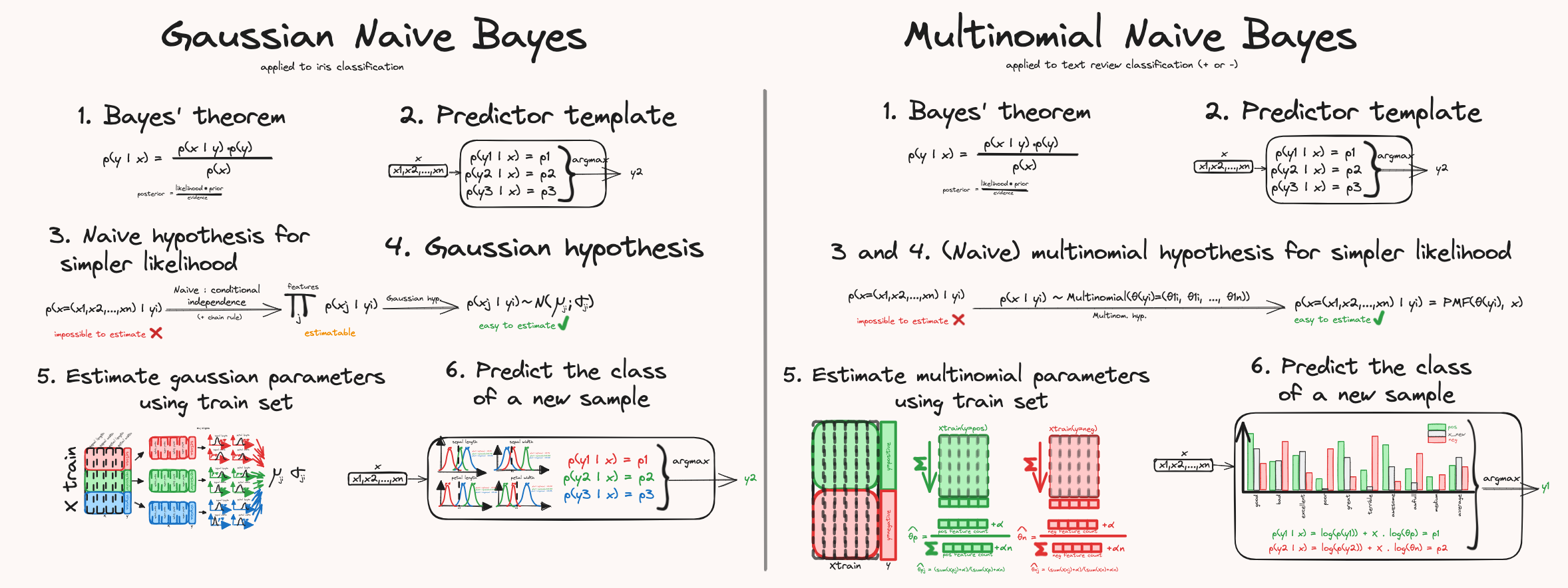
Multinomial Naive Bayes Classifier

In this new post, we are going to try to understand how multinomial naive Bayes classifier works and provide working examples with Python and scikit-learn.

What we'll see:

• What is the multinomial distribution: As opposed to Gaussian Naive Bayes classifiers that rely on assumed Gaussian distribution, multinomial naive Bayes classifiers rely on multinomial distribution.
• The general approach to create classifiers that rely on Bayes theorem, together with the naive assumption that the input features are independent of each other given a target class.
• How a multinomial classifier is "fitted" by learning/estimating the multinomial probabilities for each class – using the smoothing trick to handle empty features.
• How the probabilities of a new sample are computed, using the log-space trick to avoid underflow.

All images by author.

Understanding the multinomial distribution

If you are already familiar with the multinomial distribution, you can move on to the next part.

The first important step to understand the Multinomial Naive Bayes classifier is to understand what a multinomial distribution is.

In simple words, it represents the probabilities of an experiment that can have a finite number of outcomes and that is repeated N times, for example, like rolling a dice with 6 faces say 10 times and counting the number of times each face appears. Another example is counting the number of occurence each word in a vocabulary appear in a text.

You can also see the multinomial distribution as an extension of the binomial distribution: except for tossing a coin with 2 possible outcomes (binomial), you roll a dice with 6 outcomes (multinomial). As for the binomial distribution, the sum of all the probabilities of the possible outcomes must sum to 1. So we could have:

• for the binomial distribution of a fair coin: p(heads)+p(tails)=0.5+0.5=1
• for the binomial distribution of a loaded coin: p(heads)+p(tails)=0.3+0.7=1
• for the multinomial distribution of a fair dice: p(1)+p(2)+…+p(6)=1/6+1/6+…+1/6=1
• for the multinomial distribution of a loaded dice: p(1)+p(2)+…+p(6)=1/6+1/4+1/4+1/6+1/12+1/12=1

We can emulate such a distribution using numpy random choice function. For example, to sample 100 samples from the loaded dice distribution:

loaded_dice_probs = [1/6, 1/4, 1/4, 1/6, 1/12, 1/12]
dice_faces = [1, 2, 3, 4, 5, 6]
n_try = 100
# Sample the distribution
sampled_loaded_dice = np.random.multinomial(n_try, loaded_dice_probs)
sampled_loaded_dice
#--> array([17, 26, 21, 18,  8, 10])

Another important thing to know about the multinomial distribution is the Probability mass function. The probability mass function gives the probability to observe a specific result from a discrete distribution. For 100 tosses for the loaded coin, the probability to get 64 heads and 36 tails is:

which is actually just the binomial law (2-multinomial law). For a multinomial law, we get a generalized expression for multinomial probabilities (p_1, …, p_n) and a total number of tries N=x_1+…+x_n:

So say we have a loaded dice and we want to assess the probability that this dice's distribution is (1/6,1/4,1/4,1/6,1/12,1/12). To do so, we throw the dice say 100 times, and get x1=12 face 1, x2=15 face 2, and so on. Then we can compute the probability to observe such a result:

Hence, this example shows how to compute the probability to observe a given result (all the xi's) given associated probabilities (all the pi's). This is important since it will help compute the probability that a given sample X=(x1,…,xn) belongs to a possible multinomial distribution p=(p1,…,pn) in our classification problem.

Multinomial approach for classification

Gaussian Naive Bayes and Multinomial Naive Bayes are actually pretty close in their rationale, and mostly differ in the assumption of the underlying features distributions: instead of assuming that each feature, for each class, follows a Gaussian distribution, we assume they follow a multinomial distribution.

If you haven't read it already, I highly recommend reading my post about Gaussian naive Bayes classifier post:

Naive Bayes clearly explained

Compared to the Gaussian approach, the way the distribution parameters are estimated is different during the learning process, as well as the way they are used in the prediction process. But overall, the process is really similar. Just to give you a quick reminder, here are the important steps:

1. State Bayes theorem that allows us to compute the probability that a sample belongs to a given class y.
2. Create an empty classifier that consists of computing the probability a new sample belongs to all classes and return the class with the biggest probability.
3. and 4. To be able to compute the probabilities of Bayes equation, we do the following: discard the denominator p(x) since it does not matter when comparing each class – then we need to simplify the likelihood term using the assumption that the features altogether follow a multinomial distribution, for each class (the naive independence is actually built-in the multinomial distribution). We can then use the probability mass function of the multinomial distribution to compute the probability that a given sample belongs to a class.
4. We then have all the tools to fit our model, by learning the multinomial distribution parameters, for each class.
5. Once the model is fitted, we can use the pmf to compute the final probabilities given by Bayes theorem and return the highest probability class.

For a deeper explanation of the first 2/3 steps, see the article about Gaussian Naive Bayes classifier.

Let's quickly review the terms in Bayes equation left at step 3:

where p(y_i) is the probability that any sample belongs to class y_i, which is simply given by the proportion of each class in the dataset – and p(x|y_i) is the probability that a sample is equal to x, given it belongs to class y_i: this is exactly what the PMF gives us. In other words, the probability that a sample x belongs to class y_i is:

where p_1i is the multinomial probability associated with feature 1, for class i.

Now, just like we removed the denominator from Bayes equation, we can remove the leading fraction for the PMF, since it also only depends on x and not the class, so we end up with:

This means that we only need to estimate the multinomial probabilities for each class, and we'll be able to compute the probability a sample belongs to any class.

Note that we did not need to use the chain rule and independence assumption the same way we did for the Gaussian approach. Another way to represent this in terms of a product of independent probability terms is to write:

Estimate multinomial parameters, using smoothing trick

Now that we know how we are going to compute the probabilities that a given sample belongs to a class yi, we need to estimate the multinomial probability parameters, both for the positive and negative distribution.

To do so, we are going to use part of the dataset, namely the "training set," to train our model so it "learns" those multinomial parameters. This part explains how it does numerically.

The first and easiest step is to compute the class priors, i.e., the probability to observe a class yi (irrespective of the sample x). This is done by computing the proportions of each class in the training set.

The next step is to compute the multinomial parameters (pj's both for pos and neg). Each class is handled independantly from the other. For each class, the X training set is summed over all samples, so we compute a vector of "feature count": the idea is that this vector distribution is an image of the true underlying distribution. Then to transform those vector of feature count into a "valid" vector of multinomial distribution parameter, we divide this vector by the total sum.

But what if a word never appears in a class, like the word "atrocious" never appears in the positive part of the training set? Then the associated probability θ_atrocious for the positive class would be 0 (the numerator would be 0), which would lead to the overall probability that this sample belongs to the positive class being 0 as well:

In other words, the mere fact that the word "atrocious" was never seen in the learning process means that any new sample will have a probability of 0 to belong to the positive class, irrespective of the content of that new sample.

Put another way, we cannot allow any of the multinomial distribution probability parameters to be 0 for any class; otherwise, the total Bayes probability will always be 0 for that class.

To avoid such a situation, we use the "smoothing trick," which consists of adding an α term both to the numerator and denominator when estimating the probability parameters. This way, even if a feature (a word) is absent for all samples, the estimated-learned probability won't be 0:

Now that we know how the multinomial probabilities parameters are estimated properly, we can move onto predicting the class of a new sample.

Compute predictions, in log-space to avoid numerical underflow

Now that we have all the values needed to compute the probabilities that each sample belong to any class, we can plug the numbers in and execute the computation to predict the class.

Say the input dataset contains 1000 or 10000 columns (think of all the words in the document's vocabulary), with lots of words that appear very sparsely making their probability very small. How would this translate into the computation of the total probability for a given class y:

where x_j is the value of sample x at column j, and p_j is the probability of the multinomial distribution parameter j for that class.

Let's simulate this by creating a dataset of 300 samples of 10000 feature columns, with values between 1 and 50. In the text context, this corresponds to 300 documents with a vocabulary of 100000 words, where each word in each document appears between 1 and 50 times.

import numpy as np
J = 10000
nsamples = 300
X = np.random.choice(np.arange(1, 50), size=(nsamples,J)) 
# split into train and test (test has only 1 sample)
X_train, X_test = X[:-1], X[-1]
# estimate the distribution probabilities
feature_probs = X_train.sum(axis=0)/ X_train.sum()
print(feature_probs)
# [9.53780825e-05 1.05477725e-04 1.03631698e-04 ... 1.07925718e-04
# 1.09517582e-04 9.51506733e-05]

As you can see, the corresponding probabilities are of the order of 1e-4, which is small but computers are used and prepared to deal with such numbers, so no problem for now. But troubles appear when computing the probability that a sample belongs to a class, which is obtained as seen above by taking the product of all p_j^{x_j}, where p_j is the estimated probability for word j, and x_j is the number of occurrences of word j in the test sample. We then get:

# compute the probability for the test sample
print(feature_probs ** X_test)
print(np.prod(feature_probs ** X_test))
[1.37037886e-169 2.34731879e-064 5.34752484e-188 ... 1.84077019e-032
 1.72545280e-024 4.29538125e-069]
0.0

The individual terms of the product are between 1e-24 and 1e-188, which is very, very (very!) small and already in the orders of magnitudes regular computers and numerical packages like numpy can have trouble dealing with. Computing the overall product of those numbers (so 10000 terms product of already tiny values), we definitely go below what our computer can deal with, and end up with what Python recognizes as 0. In other words, from a product that contains no 0, we end up with 0. And that would be the case for all classes y, making the final comparison to select the most likely class impossible.

This problem is known as numerical underflow, where variables values are so close to 0 that we lose any precision and relative order between them.

To circumvent this underflow problem, the trick is to do all computations in a "log space", because the log of a small value is just a negative value but not small (not that close to 0). The general idea is to take the log of our quantities And since the logarithm function provides useful properties, we can even rewrite the formulas:

So for example the probability that a sample x belong to class y was:

becomes:

In other words, we went from a huge product of very small values, to a weighted sum of (regular) negative values. Note that this works only because log is monotonic (so partial order is conserved).

The following image sums up the computation process in log space to predict the class of a new sample:

Python example for multinomial Naive Bayes

Let's first create a toy dataset of words using known distributions. We are going to use a text classification example, but this could apply to anything else; it is just well-suited and a textbook example for this model.

Picture this as a classification problem where we want to sort reviews of customers using a bag-of-words approach for predefined 10 words: this means that a review corresponds to a row sample, and features represent the number of times each word appears in the review. In the real world, this dataset would be the output of your data extraction and preprocessing.

As the first step, we generate 2 multinomial distributions:

import numpy as np
import pandas as pd
import matplotlib.pyplot as plt
import seaborn as sns
from sklearn.feature_extraction.text import CountVectorizer
from sklearn.model_selection import train_test_split
from sklearn.naive_bayes import MultinomialNB

# Define the vocabulary
vocabulary = ['good', 'bad', 'excellent', 'poor', 'great', 'terrible', 'awesome', 'awful', 'fantastic', 'horrible']
# here the learned vocabulary is set from the begining
# it is usually created with the dataset but for this we assume it is limited to this list

# Define probabilities for positive distribution
# note that probabilities for "bad" words are not 0, so they might appear in positive docs, and vice versa
# also, normalize probabilities to sum to 
positive_probs = np.array([0.3, 0.1, 0.5, 0.1, 0.4, 0.1, 0.6, 0.1, 0.5, 0.1])
negative_probs = np.array([0.1, 0.3, 0.1, 0.5, 0.1, 0.4, 0.1, 0.6, 0.1, 0.5])
positive_probs /= positive_probs.sum()
negative_probs /= negative_probs.sum()

# Let's plot each distribution
df = pd.DataFrame({'neg': negative_probs, 'pos': positive_probs},index=vocabulary)
df_melted = df.reset_index(names='word').melt(id_vars='word', value_vars=['pos', 'neg'], var_name="class", value_name="prob.")
g = sns.catplot(df_melted, y="prob.", hue="class", x='word', kind='bar')
g.ax.set_xticklabels(g.ax.get_xticklabels(), rotation=90, ha='center', va='top')
g.ax.set_title('True distrbutions')

So for now we just created 2 multinomial distributions. It is time to use them and sample them to create an actual dataset, with known classes.

# Generate random documents for each class
# create 1000 positive reviews and 1000 negative reviews : our dataset is balanced
# the length (=number of words=sum of each row) may vary between 5 and 15 words)
# note that the vocabulary of each review (=number of distinct word) may be different
n_samples = 1000
positive_docs = [' '.join(np.random.choice(vocabulary, size=np.random.randint(5, 15), p=positive_probs)) for _ in range(n_samples)]
negative_docs = [' '.join(np.random.choice(vocabulary, size=np.random.randint(5, 15), p=negative_probs)) for _ in range(n_samples)]

# Create labels
labels_positive = np.ones(n_samples, dtype=int)
labels_negative = np.zeros(n_samples, dtype=int)

# Combine documents and labels
documents = np.concatenate([positive_docs, negative_docs])
labels = np.concatenate([labels_positive, labels_negative])

plt.figure()
sns.heatmap(CountVectorizer(vocabulary=vocabulary).fit_transform(documents).toarray(), xticklabels=vocabulary, cbar_kws={'label':'word count'})#, cmap="copper")

As you can see, we generated 2000 samples with 1000 samples sampled from the positive multinomial distribution and 1000 from the negative one. The actual "reviews" (list of words) are converted into a numerical matrix using the CountVectorizer of scikit-learn (in essence equivalent to the standard collections.Counter). In other words, we have our input dataset X with corresponding target class vector y. In practice, your work starts here with a given dataset from the real world.

We can first manually estimate the distribution parameters, kinda what scikit-learn multinomial model does when using .fit. As explained above, scikit-learn actually works in the "log-space", and the probabilities are not available as is. We can compute the learned probabilities simply using thetas = (classifier.featurecount.T / classifier.featurecount.sum(axis=1)).T.

X_train, X_test, y_train, y_test = train_test_split(documents, labels, test_size=0.2, random_state=42, shuffle=True)

# Create a CountVectorizer to convert documents into a matrix of token counts
vectorizer = CountVectorizer(vocabulary=vocabulary)

# Fit and transform the training data
X_train_counts = vectorizer.fit_transform(X_train)

# Train a multinomial naive Bayes classifier
classifier = MultinomialNB(alpha=0)  # notice I use alpha=0 here because I control the dataset and know there are no "empty" feature
classifier.fit(X_train_counts, y_train)
for class_, count_, feature_count_ in zip(classifier.classes_, classifier.class_count_, classifier.feature_count_):
    print("For class", class_, "there were ", count_, "instance in the dataset. For those samples, the total counts for each word is", feature_count_)

# estimate distribution parametsers ourselves from scikit-learn stored attributes
thetas = (classifier.feature_count_.T / classifier.feature_count_.sum(axis=1)).T
print(thetas)
# sort by class
X_train_pos = X_train_counts[y_train==0]
X_train_neg = X_train_counts[y_train==1]
print(X_train_pos.sum(axis=0)/X_train_pos.sum(), X_train_neg.sum(axis=0)/X_train_neg.sum())

df = pd.DataFrame({'neg': thetas[0], 'pos': thetas[1]}, index=vocabulary)
df_melted = df.reset_index(names='word').melt(id_vars='word', value_vars=['pos', 'neg'], var_name="class", value_name="prob.")
g = sns.catplot(df_melted, y="prob.", hue="class", x='word', kind='bar')
g.ax.set_xticklabels(g.ax.get_xticklabels(), rotation=90, ha='center', va='top')
g.ax.set_title('Learned distrbutions')

For class 0 there were  799.0 instance in the dataset. For those samples, the total counts for each word is [ 258.  815.  256. 1274.  294. 1134.  296. 1618.  264. 1402.]
For class 1 there were  801.0 instance in the dataset. For those samples, the total counts for each word is [ 827.  277. 1306.  281. 1121.  293. 1618.  228. 1344.  244.]
[[0.03389831 0.10708186 0.03363553 0.1673893  0.0386283  0.14899488
  0.03889108 0.21258705 0.03468664 0.18420707]
 [0.10969625 0.03674227 0.17323252 0.03727285 0.14869346 0.03886457
  0.21461732 0.03024274 0.17827298 0.03236504]]
[[0.03389831 0.10708186 0.03363553 0.1673893  0.0386283  0.14899488
  0.03889108 0.21258705 0.03468664 0.18420707]] 
[[0.10969625 0.03674227 0.17323252 0.03727285 0.14869346 0.03886457
  0.21461732 0.03024274 0.17827298 0.03236504]]

Since our training set contains a lot of samples, the learned distributions are pretty close to the true ones used to generate them.

A way to understand how multinomial classification works here is to compare the distribution of candidate classes along the sample's distribution. Roughly speaking, the classifier returns the class whose distribution looks the most like the sample's one:

x_new = vectorizer.transform(X_test)[0].toarray()[0]
x_normed = x_new / x_new.sum()

df = pd.DataFrame({'neg': thetas[1], 'pos': thetas[0], 'new':x_normed}, index=vocabulary)
df_melted = df.reset_index(names='word').melt(id_vars='word', value_vars=['pos', 'new', 'neg'], var_name="class", value_name='prob.')
g = sns.catplot(df_melted, y="prob.", hue="class", x='word', kind='bar')
g.ax.set_xticklabels(g.ax.get_xticklabels(), rotation=90, ha='center', va='top')
g.ax.set_title('Learned distrbutions along with new sample to predict')

For this sample, we would visually predict positive. But let's use scikit-learn model provide a numerical-based decision:

classifier.predict([x_new])
#--> array([0]) 

Finally, we can inspect and try to reproduce manually the computations made by the model in the log-space. Note that when you use .predict_proba on the model, it just takes the exponential of the log-probs:

x_new = [vectorizer.transform(X_test)[0].toarray()[0]]

# class log prior
print(classifier.class_log_prior_)
print(np.log(classifier.class_count_/classifier.class_count_.sum()))

# feature log 
print(classifier.feature_log_prob_)
print(np.log(classifier.feature_count_.T / classifier.feature_count_.sum(axis=1)).T)

# final log  likelihood
print(classifier.predict_joint_log_proba(x_new))
jll = np.dot(x_new, np.log(classifier.feature_count_.T / classifier.feature_count_.sum(axis=1))) + np.log(classifier.class_count_/classifier.class_count_.sum())
print(jll)

# log prob.
print(classifier.predict_log_proba(x_new))
from scipy.special import logsumexp
log_prob_x = logsumexp(jll, axis=1) 
print(jll - np.atleast_2d(log_prob_x).T)
# last 3 lines are equivalent to normalizing the sum of probability in 'not-log-space': x_ = x_ / x_.sum()

# final prob
print(classifier.predict_proba(x_new))
print(np.exp(jll - np.atleast_2d(log_prob_x).T))

# actual source code around https://github.com/scikit-learn/scikit-learn/blob/5c4aa5d0d90ba66247d675d4c3fc2fdfba3c39ff/sklearn/naive_bayes.py#L105

[-0.69439796 -0.69189796]
[-0.69439796 -0.69189796]
[[-3.38439026 -2.23416174 -3.3921724  -1.78743301 -3.25377008 -1.90384336
  -3.24699039 -1.54840375 -3.36140075 -1.69169478]
 [-2.21004013 -3.30382732 -1.75312052 -3.28949016 -1.9058684  -3.24767222
  -1.53889873 -3.4984992  -1.72443931 -3.4306766 ]]
[[-3.38439026 -2.23416174 -3.3921724  -1.78743301 -3.25377008 -1.90384336
  -3.24699039 -1.54840375 -3.36140075 -1.69169478]
 [-2.21004013 -3.30382732 -1.75312052 -3.28949016 -1.9058684  -3.24767222
  -1.53889873 -3.4984992  -1.72443931 -3.4306766 ]]
[[-16.67116009 -20.94229983]]
[[-16.67116009 -20.94229983]]
[[-0.01386923 -4.28500897]]
[[-0.01386923 -4.28500897]]
[[0.9862265 0.0137735]]
[[0.9862265 0.0137735]]

Remember that we used alpha=0 to easily reproduce computations by hand, but as this is a hyperparameter, it'd probably be tuned (as well as the preprocessing step to convert your raw data to a well formatted dataset).

Wrap-up

Here's what you should remember from this post:

• Multinomial distribution represent experiment that can have N different outputs and are repeated M times. Think of it as a generalisation of the binomial distribution of the coin toss, like counting each face for a dice thrown repeteadly
• The overall idea of Multinomial naive Bayes classifier is really similar to that of Gaussian naive Bayes classifier, and only differ in the fitting and predicting computations. An important thing to remember is also the underlying assumption that your features follow one of those distributions
• In order to learn the multinomial probability parameters for each class, we simply sum the training set along features, and divide the result by the sum of that vector. This provides for estimations of the probabilities. Using a smoothing term takes care for empty features ("atrocious" never appear in positive reviews for example).
• To predict the class of a new sample, we use the probability mass function of multinomial distribution, and compute all probabilities in a "log-space" in order to avoid underflow and ridiculously small numbers our computer wouldn't handle.

---

If you like this post, please give it a good round of clap and check some of my other posts:

Sklearn tutorial

Data science and Machine Learning

Fourier-transforms for time-series

Scientific/numerical python

Tags: Bayesian Machine Learning Data Science Deep Dives Probability Scikit Learn

Comment