Neural Networks For Periodic Functions

Author:Murphy | View: 22126 | Time: 2025-03-22 23:15:33

Photo by Willian Justen de Vasconcellos on Unsplash

Neural networks are known to be great approximators for any function – at least whenever we don't move too far away from our dataset. Let us see what that means. Here is some data:

It does not only look like a sine wave, it actually is, with some noise added. We can now train a normal feed-forward neural network having 1 hidden layer with 1000 neurons and ReLU activation. We get the following fit:

It looks quite decent, apart from the edges. We could fix this by adding more neurons to the hidden layer according to Cybenko's universal approximation theorem. But I want to point you something else:

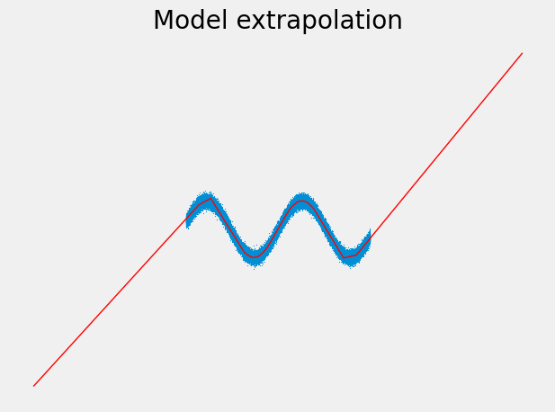
We could argue now that this extrapolation behavior is bad if we assume the wave pattern to continue outside of the observed range. But if there is no domain knowledge or more data we can resort to, it would just be this: an assumption.

However, in the remainder of this article, we will assume that any periodic pattern we can pick up within the data continues outside as well. This is a common assumption when doing time series modeling, where we naturally want to extrapolate into the future. We assume that any observed seasonality in the training data will just continue like that, because what else can we say without any additional information? In this article, I want to show you how using sine-based activation functions helps bake this assumption into the model.

But before we go there, let us shortly dive deeper into how ReLU-based neural networks extrapolate in general, and why we should not use them for time series forecasting as is.

Extrapolation of Neural Networks

We have seen that the output of our ReLU network turns into a line the further we go away from our dataset. This is a general pattern, as shown by Ziyin et al. in their paper Neural Networks Fail to Learn Periodic Functions and How to Fix It. They prove:

To simplify it a little bit, you can read it as f(z·u) ≈ z·W·u + b for large z. This shows that if you plug in absolutely large values in the ReLU neural network – meaning very far away from 0 – this network behaves like a linear function.

If the input and output are one-dimensional, such as in our example, we can set u = 1 and get f(z) ≈ W·z + b for large z, where W is a 1×1 matrix, i.e., a real number. Setting u = -1, we get f(-z) ≈ W'·z + b for large z and some other number W'. This is exactly what we have seen on the edges.

Sigmoid- or tanh-based networks

Something similar holds for bounded activation functions such as sigmoid or tanh:

The authors formalize it in

This means that our model behaves like a constant function f(z·u) ≈ v whenever we go away far from 0, as opposed to a more general linear function in the ReLU case.

While this is all interesting, let us get to the activation functions that can model periodic behavior.

Sine-Based Activation Functions

There are several ways to proceed from here. The easiest thing is just to use sin(x) as an activation function and see what happens. Ziyin et al. put even more thought into it and suggest using their so-called snake function Snake(x) = x + sin²(x), or even Snakeₐ(x) = x + sin²(ax) / a, __ if you want to parameterize it.

Pure sine

Let us build a model using only a single hidden note with the sine function as the activation. I will use TensorFlow to implement it, but it is so simple that you can use any Deep Learning framework to follow along.

import tensorflow as tf

model = tf.keras.Sequential([
    tf.keras.layers.Dense(1, activation=tf.math.sin),
    tf.keras.layers.Dense(1)
])

model.compile(
    loss="mse",
    optimizer=tf.keras.optimizers.AdamW() # AdamW is a better version of Adam, see here: https://arxiv.org/abs/1711.05101
)

We can now train the model:

X = tf.random.uniform((100000, 1), minval=-6, maxval=6)
y = tf.math.sin(X) + 0.1 * np.random.randn(100000, 1)

model.fit(
    X,
    y,
    validation_split=0.1,
    epochs=100,
    callbacks=[
        tf.keras.callbacks.EarlyStopping(patience=2, restore_best_weights=True), # stop whenever the validation mse does not improve in two epochs
        tf.keras.callbacks.ReduceLROnPlateau(patience=0) # lower learning rate if the validation mse does not improve
    ]
)

We get the following fit:

This is what we would like to see when doing a time series forecast! Although the left side (the past) usually does not matter, it is nice to get a reasonable extrapolation there as well for free.

A word of caution. Do not throw in too many hidden nodes, since otherwise, the model might pick up seasonalities that do not exist in the data – classical overfitting. Look at what can happen if we use 100 hidden nodes:

In addition to the short seasonality, the model picks up a larger seasonality that goes down in the time of the training. We know that this is not true, though, for our data.

Less is more.

Snake function

The authors did not invent the snake function for stationary data as we have it at the moment. It will not work well with our data since it imposes a trend on the model.

def snake(x):
    return tf.math.sin(x)**2 + x

model = tf.keras.Sequential([
    tf.keras.layers.Dense(5, activation=snake),
    tf.keras.layers.Dense(1)
])

Training this model gives something like this:

We can see an upward trend that also comes out of nowhere. But this is a consequence of how the snake function is designed, i.e., the "+ x" term. For functions or time series with a trend, though, the snake function can shine.

The authors also present a universal extrapolation theorem:

From their paper. C¹ functions have continuous first derivatives.

This is similar to the Fourier approximation theorem, but not the same since we use the snake function here, instead of pure sine and cosine waves.

Time Series With a Trend

Let us say that we want to forecast a time series now, and we assume that it

has potentially many seasonalities, such as hourly, monthly, yearly, or even some period we cannot easily describe, and
a trend.

There are a lot of classical statistical methods to tackle this problem, such as SARIMA or triple exponential smoothing, also known as Holt-Winters. On the neural network side, you can use recurrent Neural Networks, convolutions, or transformers.

However, I will not go into the details of these methods but focus on our main goal: building simple sine-based feed-forward neural networks. In contrast to many of the aforementioned methods, we do not have to deal with recursive formulas in this case but model our target directly. Let us first create some data we can train on.

X = tf.cast(tf.range(50)[:, tf.newaxis], tf.float32)
y = 3*tf.math.sin(X) + 2*tf.math.sin(2*X) - tf.math.sin(3*X) + X + 0.1 * tf.random.normal((50, 1))

The data looks like this:

Additive trend + seasonality model

We can implement it in keras like this:

class AdditiveTrendAndSeasonalityModel(tf.keras.Model):
    def __init__(self, trend_model, seasonality_model):
        super().__init__()
        self.trend_model = trend_model
        self.seasonality_model = seasonality_model

    def call(self, x):
        return self.trend_model(x) + self.seasonality_model(x)

trend_model = tf.keras.Sequential([
    tf.keras.layers.Dense(5, activation="relu"),
    tf.keras.layers.Dense(1)
])

seasonality_model = tf.keras.Sequential([
    tf.keras.layers.Dense(5, activation=tf.math.sin),
    tf.keras.layers.Dense(1, use_bias=False)
])

model = AdditiveTrendAndSeasonalityModel(trend_model, seasonality_model)

Now we can compile and train the model.

model.compile(
    loss="mse",
    optimizer=tf.keras.optimizers.AdamW(learning_rate=0.0005)
)

model.fit(
    X,
    y,
    epochs=3000,
    callbacks=[tf.keras.callbacks.EarlyStopping(monitor="loss", patience=5)]
)

We can use our model to extrapolate now:

The extrapolation behavior of our model looks great! The trend is nice and linear, just as in the training data, but the seasonality pattern could be more accurate. The pattern that the model came up with is too simple, although the model had the chance to learn the true pattern since we gave it five sine-activated nodes. Only three would have been necessary.

I also experienced that initialization matters very much in sine-based neural networks. Sometimes, we get a good and fast convergence to a model as in the image above. But sometimes, we get stuck in very bad local minima – it is a bit of a hit-and-miss.

Still, since our model consists of a trend_model and seasonality_model , we can easily decompose our time series into a trend and seasonal part:

Nice! And if you want a multiplicative trend, just replace the + with a * in the model class.

Conclusion

In this article, we have seen that the extrapolation capabilities of neural networks are determined by their activation functions – a fact that many people are not aware of.

Furthermore, for time series modeling, we have seen how to create a simple neural network that consists of a trend and seasonality part that are then added together, giving us a nice decomposition. And because we are dealing with time series, extrapolation capabilities are crucial. Hence we have to be careful which activation functions we choose. In the case of the seasonality part of our network, we used sine activation functions since they make this part of the neural network periodic.

You can also use the snake function that Ziyin et al. proposed, but then you will lose the ability to decompose the time series into trend and seasonality components. But give it a try, if this is not important to you, and rather the predictive performance matters.

I hope that you learned something new, interesting, and valuable today. Thanks for reading!