Running SQL Queries in Jupyter Notebook using JupySQL, DuckDB, and MySQL

Traditionally, data scientists use Jupyter Notebook to pull data from database servers, or from external datasets (such as CSV, JSON files, etc) and store them into Pandas dataframes:

They then use the dataframes for visualization purposes. This approach has a couple of drawbacks:

• Querying a database server may degrade the performance of the database server, which may not be optimized for analytical workloads.
• Loading the data into dataframes take up precious resources. For example, if the intention is to visualize certain aspects of the dataset, you need to first load the entire dataset into memory before visualization can be performed.

To improve the performance of the above, ideally the processing of the data (all the data wrangling and filtering) should be offloaded to a client which is able to perform the data analytics efficiently, and return the result to be used for visualization. And this is the topic of this article – JupySQL.

JupySQL is a SQL client for Jupyter Notebook, allowing you to access your datasets directly in Jupyer Notebook using SQL. The main idea of JupySQL is to run SQL in a Jupyter Notebook, hence its name.

JupySQL allows you to query your dataset using SQL, without needing you to maintain the dataframe to store your dataset. For example, you could use JupySQL to connect to your database server (such as MySQL or PostgreSQL), or your CSV files through the Duckdb engine. The result of your query can then be directly used for visualization. The following figure shows how JupySQL works:

You can use the following magic commands to use Jupysql in your Jupyter Notebooks:

• %sql – this is a line Magic Command to execute a SQL statement
• %%sql – this is a cell magic command to execute multiple-line SQL statements
• %sqlplot – this is a line magic command to plot a chart

Our Datasets

For this article, I am going to use a few datasets:

• Titanic Dataset (_titanictrain.csv). Source: https://www.kaggle.com/datasets/tedllh/titanic-train. Licensing – Database Contents License (DbCL) v1.0
• Insurance Dataset (insurance.csv). Source: https://www.kaggle.com/datasets/teertha/ushealthinsurancedataset. Licensing – CC0: Public Domain.
• 2015 Flights Delay Dataset (airports.csv). Source: https://www.kaggle.com/datasets/usdot/flight-delays. Licensing – CC0: Public Domain
• Boston Dataset (boston.csv). Source: https://www.kaggle.com/datasets/altavish/boston-housing-dataset. Licensing – CC0: Public Domain
• Apple Historical Dataset (AAPL.csv). Source: (https://www.kaggle.com/datasets/prasoonkottarathil/apple-lifetime-stocks-dataset). License – CC0: Public Domain

Installing JupySQL

To install the JupySQL, you can use the pip command:

!pip install jupysql duckdb-engine --quiet

The above statement installs the jupysql package as well as the duckdb-engine.

Next step is to load the sql extension using the %load_ext line magic command:

%load_ext sql

Integrating with DuckDB

With the sql extension loaded, you need to load a database engine in which you can use it to process your data. For this section, I am going to use DuckDB. The following statement starts a DuckDB in-memory database:

%sql duckdb://

Performing a query

With the DuckDB database started, let's perform a query using the airports.csv file:

%sql SELECT * FROM airports.csv ORDER by STATE

You will see the following output:

If your SQL query is long, use the %%sql cell magic command:

%%sql
SELECT 
    count(*) as Count, STATE 
FROM airports.csv 
GROUP BY STATE 
ORDER BY Count 
DESC LIMIT 5

The above SQL statement generates the following output:

Saving Queries

You can also use the--save option to save the query so that it can be used later:

%%sql --save boston 
SELECT 
    * 
FROM boston.csv

If you want to save a query without executing it, use the --no-execute option:

%%sql --save boston --no-execute
SELECT 
    * 
FROM boston.csv

The above statements saved the result of the query as a table named boston. You will see the following output:

*  duckdb://
Skipping execution...

Plotting

JupySQL allows you to plot charts using the %sqlplot line magic command.

Histogram

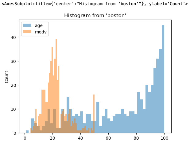
Using the saved query in the previous section, you can now plot a histogram showing the distribution of the age and medv fields:

%sqlplot histogram --column age medv --table boston --with boston

Here is the histogram showing the distribution of values for the age and medv fields:

Here's another example. This time round, we will use the titanic_train.csv file:

%%sql --save titanic 
SELECT 
   *
FROM titanic_train.csv WHERE age NOT NULL AND embarked NOT NULL

You can now plot the distribution of ages for all the passengers:

%sqlplot histogram --column age --bins 10 --table titanic --with titanic

You can specify the number of bins you want using the --bin option.

You can also customize the plot by assigning the plot to a variable, which is of type matplotlib.axes._subplots.AxesSubplot:

ax = %sqlplot histogram --column age --bins 10 --table titanic --with titanic
ax.grid()
ax.set_title("Distribution of Age on Titanic")
_ = ax.set_xlabel("Age")

Using the matplotlib.axes._subplots.AxesSubplot object, you can turn on the grid, set a title, as well as set the x-label for the plot:

Box plot

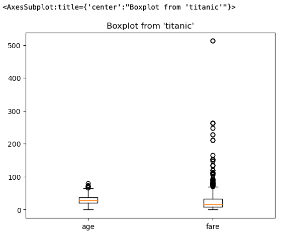
Besides histogram, you can also plot box plots:

%sqlplot boxplot --column age fare --table titanic --with titanic

The resultant box plot shows the median, minimum, and maximum values as well as outliers for both the age and fare fields:

You can also view the boxplots for the sibsp and parch fields:

%sqlplot boxplot --column sibsp parch --table titanic --with titanic

Pie chart

You can also plot pie charts using JupySQL's legacy plotting API. For this example, I am going to use the airports.csv file to find the number of airports belonging to each state.

First, I use SQL to count all the airports from each state and filter the top five:

airports_states = %sql SELECT count(*) as Count, STATE FROM airports.csv GROUP BY STATE ORDER BY Count DESC LIMIT 5
print(type(airports_states))

The result of the %sql statement is a sql.run.ResultSet object. From this object, I can obtain the dataframe if I want to:

airports_states.DataFrame()

I can also use it to call the pie() API to plot a pie chart:

import seaborn
# https://seaborn.pydata.org/generated/seaborn.color_palette.html
palette_color = seaborn.color_palette('pastel')

total = airports_states.DataFrame()['Count'].sum()
def fmt(x):    
    return '{:.4f}%n({:.0f} airports)'.format(x, total * x / 100)

airports_states.pie(colors=palette_color, autopct=fmt)

The plotting API also supports bar charts:

palette_color = seaborn.color_palette('husl')
airports_states.bar(color=palette_color)

And line charts using the plot() function (here I am using the AAPL.csv file):

apple = %sql SELECT Date, High, Low FROM AAPL.csv

# apple.plot() is of type matplotlib.axes._subplots.AxesSubplot
apple.plot().legend(['High','Low'])

Integrating with MySQL

So far all the examples in the previous few sections were all using DuckDB. Let's now try to connect to a database server. For my example, I will use the MySQL server with the following details:

• Database – Insurance
• Table – Insurance (imported from the insurance.csv file)
• User account – user1

To connect to the MySQL server, create a SQLAlchemy URL standard connection string, in the following format: mysql://username:password@host/db

The following code snippet when run will prompt you to enter the password for the user1 account:

from getpass import getpass

password = getpass()
username = 'user1'
host = 'localhost'
db = 'Insurance'

# Connection strings are SQLAlchemy URL standard
connection_string = f"mysql://{username}:{password}@{host}/{db}"

Enter the password for the user1 account:

To connect JupySQL to the MySQL server, use the %sql line magic, together with the connection string:

%sql $connection_string

If you use the %sql line magic without any inputs, you will see the current connections (which is DuckDB and MySQL):

%sql

Let's select the Insurance table to examine its content:

%sql SELECT * FROM Insurance

And let's plot a bar chart using the bar() API:

regions_count = %sql SELECT region, count(*) FROM Insurance GROUP BY region
regions_count.bar(color=palette_color)

If you like reading my articles and that it helped your career/study, please consider signing up as a Medium member. It is $5 a month, and it gives you unlimited access to all the articles (including mine) on Medium. If you sign up using the following link, I will earn a small commission (at no additional cost to you). Your support means that I will be able to devote more time on writing articles like this.

Join Medium with my referral link – Wei-Meng Lee

Summary

I hope this article has given you a better idea of how to use JupySQL and the various ways to connect to different data sources, such as MySQL and DuckDB. Also, besides connecting to our datasets, I have also showed you how you can use JupySQL to perform visualization directly using the result of your query. As usual, be sure to give it a try and let me know how it goes for you!

Tags: Duckdb Jupysql Jupyter Notebook Magic Command Sql

Comment