Singular Value Decomposition (SVD), Demystified
Singular value decomposition (SVD) is a powerful matrix factorization technique that decomposes a matrix into three other matrices, revealing important structural aspects of the original matrix. It is used in a wide range of applications, including signal processing, image compression, and dimensionality reduction in machine learning.
This article provides a step-by-step guide on how to compute the SVD of a matrix, including a detailed numerical example. It then demonstrates how to use SVD for dimensionality reduction using examples in Python. Finally, the article discusses various applications of SVD and some of its limitations.
The article assumes the reader has basic knowledge of linear algebra. More specifically, the reader should be familiar with concepts such as vector and matrix norms, rank of a matrix, eigen-decomposition (eigenvectors and eigenvalues), orthonormal vectors, and linear projections.

Mathematical Definition
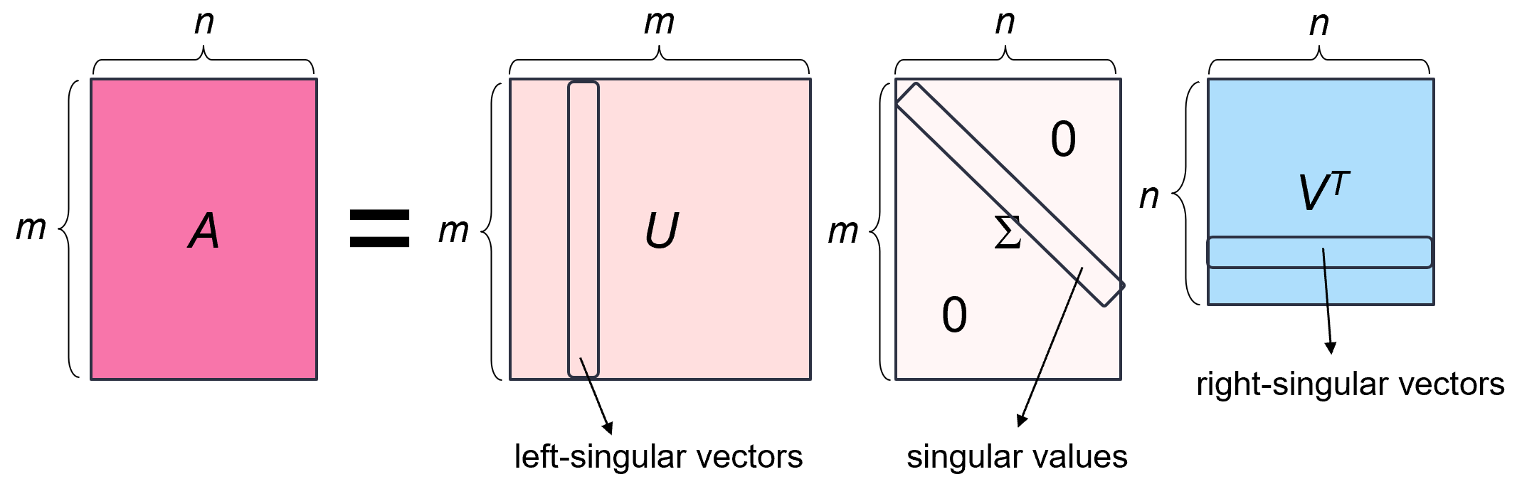
The singular value decomposition of an m × n real matrix A is a factorization of the form A = _U_ΣVᵗ, where:
- U is an m × m orthogonal matrix (i.e., its columns and rows are orthonormal vectors). The columns of U are called the left-singular vectors of A.
- Σ is an m × n rectangular diagonal matrix with non-negative real numbers on the diagonal. The diagonal entries σᵢ = Σᵢᵢ are known as the singular values of A and are typically arranged in descending order, i.e., _σ₁ ≥ σ₂ ≥ … ≥ σₙ ≥_ 0. The number of the non-zero singular values is equal to the rank of A.
- V is an n × n orthogonal matrix. The columns of V are called the right-singular vectors of A.
Every matrix has a singular value decomposition __ (a proof of this statement can be found here). This is unlike eigenvalue decomposition, for example, which can be applied only to squared diagonalizable matrices.
Computing the SVD
The singular value decomposition of a matrix A can be computed using the following observations:
- The left-singular vectors of A are a set of orthonormal eigenvectors of AAᵗ.
- The right-singular vectors of A are a set of orthonormal eigenvectors of AᵗA.
- The non-zero singular values of A are the square roots of the non-zero eigenvalues of both AᵗA and AAᵗ.
- If _U_ΣVᵗ is the SVD of A, then __ for each singular value σᵢ,

where uᵢ is the i-th column of U and vᵢ is the i-th column of V.
Proof:
- We will first show that the left-singular vectors of A are a set of orthonormal eigenvectors of AAᵗ.
Let A = _U_ΣVᵗ be the SVD of A, and let's examine __ the product _AA_ᵗ:

Since Σ is a diagonal matrix with singular values σᵢ on its diagonal, ΣΣᵗ is also a diagonal matrix where each diagonal element is _σᵢ_². Let's denote this matrix by Σ². This gives us:

Since U is orthonormal, UᵗU = I, and by right multiplying both sides of the equation by U we get:

Let's now consider a single column of U, denoted by uᵢ. Since ABᵢ = [AB]ᵢ (i.e., matrix A multiplied by column i of matrix B is equal to column i of their product AB), we can write:

Therefore, uᵢ is an eigenvector of AAᵗ corresponding to the eigenvalue λᵢ = _σᵢ_². In other words, the columns of U are eigenvectors of AAᵗ. Because the columns of U are orthonormal, the left-singular vectors of A (the columns of U) are a set of orthonormal vectors of AAᵗ.
- In a similar fashion, we can show that the right-singular vectors of A are a set of orthonormal eigenvectors of AᵗA.
- We first notice that AAᵗ is symmetric and positive semi-definite. Therefore all its eigenvalues are real and non-negative, and it has a full set of orthonormal eigenvectors. Let {u₁, …, uₙ} be the orthonormal eigenvectors of AAᵗ corresponding to eigenvalues _λ₁ ≥ λ₂ ≥ … ≥ λₙ ≥_ 0. For any eigenvector uᵢ of AAᵗ corresponding to an eigenvalue λᵢ we have:

Thus, the singular values of A are the square roots of the eigenvalues of AAᵗ.
Similarly, we can show that the singular values of A are also the square roots of the eigenvalues of AᵗA.
- Left as an exercise to the reader.
Based on the above observations, we can compute the SVD of an m × n matrix A using the following steps:
- Construct the matrix AᵗA.
- Compute the eigenvalues and eigenvectors of AᵗA. The eigenvalues will be the squares of the singular values of A, and the eigenvectors will form the columns of the matrix V in the SVD.
- Arrange the singular values of A in descending order. Create an m × n diagonal matrix Σ with the singular values on the diagonal, padding with zeros if necessary so that the matrix has the same dimensions as A.
- Normalize the eigenvectors of AᵗA to have unit length, and place them as columns of matrix V.
- For each singular value σᵢ, calculate the corresponding left-singular vector uᵢ as
where vᵢ is the i-th column of V. Place these vectors as columns in the matrix U.
If n < m or A is rank-deficient (i.e., rank(A) < min(m, n)), then there would not be enough non-zero singular values to determine the columns of U. In this case, we need to complete U to an orthogonal matrix by finding additional orthonormal vectors that span the null space (kernel) of Aᵗ.
The null space of Aᵗ, denoted N(Aᵗ), is the __ set of vectors x such that _A_ᵗx = 0, which are also the ** eigenvectors o_f AA_ᵗ corresponding to eigenvalue 0 (sinc_e A_Aᵗx = 0⋅x). To find an orthonormal basis for _N(_Aᵗ), we first solve the homogenous linear system Aᵗx =** 0 to find a basis for _N(_Aᵗ), then use the Gram-Schmidt process on this set of basis vectors to make them orthogonal, and finally we normalize them into unit vectors.
Another way to find the left-singular vectors of A (the columns of U) is to compute the eigenvectors of AAᵗ, but this process is usually more time consuming than using the relationship between the left and right singular vectors (observation 4) and computing the null space of Aᵗ (if necessary).
Note that it is also possible to start the SVD computation by finding the left-singular vectors (i.e., the eigenvectors of AAᵗ), and then use the following relationship to find the right singular vectors:

The choice of using either AAᵗ or AᵗA depends on which matrix is smaller.
Numerical Example
For example, let's compute the SVD of the following matrix:

Let _U_ΣVᵗ be the SVD of A. The dimensions of A are 3 × 2. Therefore, the size of U is 3 × 3, the size of Σ is 3 × 2, and the size of V is 2 × 2.
Since the size of AᵗA (2 × 2) is smaller than the size of AAᵗ (3 × 3), it makes sense to start with the right-singular vectors of A.
We first compute AᵗA:

We now find the eigenvalues and eigenvectors of AᵗA. The characteristic polynomial of the matrix is:


The roots of this polynomial are:

The eigenvalues of AᵗA in descending order are _λ₁ =_ 9 and _λ_₂ = 1. Therefore, the singular values of A are _σ_₁ = 3 and _σ_₂ = 1, and the matrix Σ is:

We now find the right singular vectors (the columns of V) by finding an orthonormal set of eigenvectors of AᵗA.
The eigenvectors corresponding to _λ₁ =_ 9 are:

Therefore, the eigenvectors are of the form v₁ = (t, t). For a unit-length eigenvector we need:

Thus, the unit eigenvector corresponding to _λ_₁ = __ 9 is:

Similarly, the eigenvectors corresponding to _λ_₂ = 1 are:

Therefore, the eigenvectors are of the form v₂ = (t, t). For a unit-length eigenvector we need

Thus, the unit eigenvector corresponding to _λ_₂ _ =_ 1 is:

We can now write the matrix V, whose columns are the vectors v₁ and v₂:

Lastly, we find the left-singular vectors of A. From observation 4, it follows that:


Since there is only one remaining column vector of U, instead of computing the kernel of Aᵗ, we can simply __ find a unit vector that is perpendicular to both u₁ and u₂.
Let u₃ = (a, b, c). To be perpendicular to u₂ we need a = b. Then the condition u₃ᵗu₁ = 0 becomes

Therefore,

For the vector to be unit-length, we need

Thus,

And the matrix U is:

The final SVD of A in its full glory is:

Computing SVD with NumPy
To compute the SVD of a matrix using numpy, you can call the function [np.linalg.svd](https://numpy.org/doc/stable/reference/generated/numpy.linalg.svd.html). Given a matrix A with shape (m, n), the function returns a tuple (U, S, Vᵗ), where U is a matrix with shape (m, m) containing the left- singular vectors in its columns, S is a vector of size k = min_(_m, n) containing the singular values in descending order, and Vᵗ is a matrix with shape __ (n, n) containing the right singular vectors in its rows.
For example, let's use this function to compute the SVD of the matrix from the previous example:
import numpy as np

A = np.array([[1, 0], [0, 1], [2, 2]])
np.linalg.svd(A)
The output we get is:
(array([[-2.35702260e-01,  7.07106781e-01, -6.66666667e-01],
        [-2.35702260e-01, -7.07106781e-01, -6.66666667e-01],
        [-9.42809042e-01, -1.11022302e-16,  3.33333333e-01]]),
 array([3., 1.]),
 array([[-0.70710678, -0.70710678],
        [ 0.70710678, -0.70710678]]))
This is the same SVD decomposition we have obtained with our manual computation, up to a sign difference (e.g., the first column of U has flipped direction). This shows that an SVD decomposition of a matrix is not entirely unique. While the singular values themselves are unique, the associated singular vectors (i.e., the columns of U and V) are not strictly unique due to the following reasons:
- If a singular value is repeated, the corresponding singular vectors can be chosen to be any orthonormal set that spans the associated eigenspace.
- Even if the singular values are distinct, the corresponding singular vectors can be multiplied by -1 (i.e., their direction can be flipped) and still form a valid SVD.
Compact SVD
The compact singular value decomposition is a reduced form of the full SVD, which retains only the non-zero singular values and their corresponding singular vectors.
Formally, the compact SVD of an m × n matrix A with rank r (r ≤ min{m, n}) is a factorization of the form A = _Uᵣ_ΣᵣVᵣᵗ, where:
- Uᵣ is an m × r matrix whose columns are the first r left-singular vectors of A.
- Σᵣ is an r × r diagonal matrix with the r non-zero singular values on the diagonal.
- Vᵣ is an n × r matrix whose columns are the first r right-singular vectors of A.
For example, the rank of the matrix from our previous example is 2, since it has two non-zero singular values. Therefore, its compact SVD decomposition is:

The matrices Uᵣ, Σᵣ and Vᵣ contain only the essential information needed to reconstruct the matrix A. The compact SVD can yield significant savings in storage and computation, especially for matrices with many zero singular values (i.e., when r << min{m, n}).
Truncated SVD
Truncated (reduced) SVD is a variation of SVD used for approximating the original matrix A with a matrix of a lower rank.
To create a truncated SVD of a matrix A with rank r, we take only the k < r largest singular values and their corresponding singular vectors (k is a parameter). This gives us an approximation of the original matrix Aₖ = _Uₖ_ΣₖVₖᵗ, where:
- Uₖ is an m × k matrix whose columns are the first k left-singular vectors of A, corresponding to the k largest singular values.
- Σₖ is an k × k diagonal matrix with the k largest __ singular values on the diagonal.
- Vₖ is an n × k matrix whose columns are the first k right-singular vectors of A, corresponding to the k largest singular values.

For example, we can truncate the matrix from the previous example to have a rank of k = 1 by taking only the largest single value and its corresponding vectors:

In NumPy, the truncated SVD can be easily computed using the following code snippet:
U, S, Vt = np.linalg.svd(A)

k = 1  # target rank
U_k = U[:, :k]
S_k = np.diag(S[:k])
Vt_k = Vt[:k, :]

A_k = U_k @ S_k @ Vt_k
A_k
array([[0.5, 0.5],
[0.5, 0.5],
[2. , 2. ]])Truncated SVD is particularly effective, since the truncated matrix Aₖ is the best rank-k approximation of the matrix A in terms of both the Frobenius norm (the least squares difference) and the 2-norm, i.e.,

This result is known as the Eckart-Young-Mirsky theorem or the matrix approximation lemma, and its proof can be found in this Wikipedia page.
The choice of k controls the tradeoff between approximation accuracy and the compactness of the representation. A smaller k results in a more compact matrix but a rougher approximation. In real-world data matrices, only a very small subset of the singular values are large. In such cases, Aₖ can be a very good approximation of A by retaining the few singular values that are large.
Dimensionality Reduction with Truncated SVD
Using the truncated SVD, it is also possible to reduce the number of dimensions (features) in the data matrix A. To reduce the dimensionality of A from n to k, we project the matrix rows onto the space spanned by the first k right-singular vectors. This is done by multiplying the original data matrix A by the matrix Vₖ:

The reduced matrix now has dimensions n × k and contains the projection of the original data onto the k-dimensional subspace. Its columns are the new features in the reduced dimensional space. These features are linear combinations of the original features and are orthogonal to each other.
Using our previous example, we can reduce the number of dimensions of our data matrix A from 2 to 1 as follows:

Another way to compute the reduced matrix is based on the following observation:

Proof: The full SVD of A is A = _U_ΣVᵗ, therefore AV = _U_Σ. By comparing the j-th columns of each side of the equation we get:

Therefore, all the columns of AVₖ are equal to all the columns of _Uₖ_Σₖ, so the two matrices must be equal.
Using _Uₖ_Σₖ is a more efficient way to compute the reduced matrix, because it requires to multiply matrices of size m × k and k × k, instead of matrices of size m × n and n × k (k is typically much smaller than n).
In our previous example:

Dimensionality reduction using truncated SVD is often used as a data preprocessing step before Machine Learning tasks such as classification or clustering, where it helps dealing with the curse of dimensionality, reduce computational costs and potentially improve the performance of the machine learning algorithm.
To reduce the dimensionality of new data points that arrive after the machine learning model has been trained (e.g., samples in the test set), we simply project them onto the same subspace spanned by the first k right-singular vectors of A:

Recall that our convention is to express each vector x as a column vector, while data points are stored as rows of A, which is why we left-multiply x by Vₖᵗ instead of right multiplying it by Vₖ.
Reconstruction Error
A key metric in assessing the effectiveness of dimensionality reduction techniques is called the reconstruction error. It provides a quantitative measure of the loss of information resulting from the reduction process.
To measure the reconstruction error of a specific vector, we first project it back onto the original space spanned by the m right-singular vectors. This is done by multiplying Vₖ by the reduced vector:

We then measure the reconstruction error as the mean squared error (MSE) between the reconstructed components of the vector and the original components:

We can also measure the reconstruction error of the entire matrix A by projecting the reduced matrix rows back onto the original space spanned by the m right-singular vectors. This is done by multiplying the reduced A by the transpose of Vₖ:

We can then use either the MSE between the elements of the reconstructed matrix and the original elements, or the Frobenius norm of the difference between the two matrices:

For example, the reconstructed matrix of the reduced matrix from our previous example is:

And the reconstruction error is:

Truncated SVD in Scikit-Learn
Scikit-Learn provides an efficient implementation of truncated SVD in the class [sklearn.decomposition.TruncatedSVD](https://scikit-learn.org/stable/modules/generated/sklearn.decomposition.TruncatedSVD.html). Its important parameters are:
n_components: Desired number of dimensions for the output data (defaults to 2).-
algorithm: The SVD solver to use. Can be one of the following options:'arppack'uses the ARPACK wrapper in SciPy to compute the eigen-decomposition of AAᵗ or AᵗA (whichever is more efficient). ARPACK is an iterative algorithm that efficiently computes a few eigenvalues and eigenvectors of large sparse matrices.'randomized'(the default) uses a fast randomized SVD solver based on an algorithm by Halko et al. [1].
n_iter: The number of iterations for the randomized SVD solver (defaults to 5).
For example, let's demonstrate the usage of this class on our matrix from the previous example:
from sklearn.decomposition import TruncatedSVD

svd = TruncatedSVD(n_components=1, random_state=0)
A_reduced = svd.fit_transform(A)
A_reduced
The output we get is the reduced matrix:
array([[0.70710678],
       [0.70710678],
       [2.82842712]])
Example: Image Compression
Singular value decomposition can be used for image compression. Although an image matrix is often of full rank, its lower ranks usually have very small Singular Values. Thus, truncated SVD can lead to a significant reduction in the image size without losing too much information.
For example, we will demonstrate how to use truncated SVD to compress the following image:

We first load the image into a NumPy array using the function [matplotlib.pyplot.imread](https://matplotlib.org/stable/api/_as_gen/matplotlib.pyplot.imread.html):
import matplotlib.pyplot as plt

image = plt.imread('image.jpg')
The shape of the image is:
image.shape(1600, 1200, 3)The height of the image is 1600 pixels, its width is 1200 pixels, and it has 3 color channels (RGB).
Since Svd can only be applied to 2D data, we can either execute it on each color channel separately, or we can reshape the image from a 3D matrix to a 2D matrix by flattening each color channel and stacking them horizontally (or vertically).
For example, the following code snippet reshapes the image into a 2D matrix by stacking the color channels horizontally:
height, width, channels = image.shape
flat_image = image.reshape(-1, width * channels)
The shape of the flattened image is:
flat_image.shape(1600, 3600)The rank of the image's matrix is:
np.linalg.matrix_rank(flat_image)1600The matrix is of full rank (since min(1600, 3600) = 1600).
Let's plot the first 100 singular values of the matrix:
U, S, Vt = np.linalg.svd(flat_image)

k = 100
plt.plot(np.arange(k), S[:k])
plt.xlabel('Rank of singular value')
plt.ylabel('Magnitude of singular value')
We can clearly see a rapid decay in the singular values. This decay means that we can effectively truncate the image without a significant loss of accuracy.
For example, let's truncate the image to have a rank of 100 using Truncated SVD:
svd = TruncatedSVD(n_components=100)
truncated_image = svd.fit_transform(flat_image)
The shape of the truncated image is:
truncated_image.shape(1600, 100)The size of the truncated image is only 100/3600 = 2.78% of the original image!
To see how much information was lost in the compression we can measure the image's reconstruction error. We will measure the reconstruction error as the mean of squared errors (MSE) between the the pixel values of the original image and the reconstructed image.
In Scikit-Learn, the reconstructed image can be obtained by calling the method inverse_transform of the TruncatedSVD transformer:
reconstructed_image = svd.inverse_transform(truncated_image)Therefore, the reconstruction error is:
reconstruction_error = np.mean(np.square(reconstructed_image - flat_image))
reconstruction_error29.323291415822336Thus, the root mean squared error (RMSE) between the pixel intensities in the original image and the reconstructed image is only about 5.41 (which is small relative to the range of the pixels [0, 255]).
To display the reconstructed image, we first need to reshape it into the original 3D shape and then clip the pixel values to integers in the range [0, 255]:
reconstructed_image = reconstructed_image.reshape(height, width, channels)
reconstructed_image = np.clip(reconstructed_image, 0, 255).astype('uint8')
We can now display the image using the plt.imshow function:
plt.imshow(reconstructed_image)
plt.axis('off')
We can see that the reconstruction at rank 100 loses only a small amount of detail.
Let's place all the above steps into a function that compresses a given 3D image to a specified number of dimensions and then reconstructs it:
def compress_image(image, n_components=100):
    # Reshape the 3D image into a 2D array by stacking the color channels horizontally
    height, width, channels = image.shape
    flat_image = image.reshape(-1, width * channels)

    # Truncate the image using SVD
    svd = TruncatedSVD(n_components=n_components)
    truncated_image = svd.fit_transform(flat_image)

    # Recover the image from the reduced representation
    reconstructed_image = svd.inverse_transform(truncated_image)

    # Reshape the image to the original 3D shape
    reconstructed_image = reconstructed_image.reshape(height, width, channels)

    # Clip the output to integers in the range [0, 255]
    reconstructed_image = np.clip(reconstructed_image, 0, 255).astype('uint8')
    return reconstructed_image
We can now call this function with different number of components and examine the reconstructions:
fig, axes = plt.subplots(1, 5, figsize=(10, 50))
plt.setp(axes, xticks=[], yticks=[])  # Remove axes from the subplots

for i, k in enumerate([5, 10, 20, 50, 100]):
    output_image = compress_image(image, k)
    axes[i].imshow(output_image)
    axes[i].set_title(f'$k$ = {k}')
As we can see, using a rank that is too low, such as k = 10, can lead to a substantial loss of information, while an SVD of rank 200 is almost indistinguishable from the full-rank image.
In addition to compressing images, SVD can also be used to remove noise from images. This is because discarding the lower-order components of the image tends to remove the granular, noisy elements, while preserving the more significant parts of the image.
Applications of SVD
SVD is employed in many types of applications where it helps to uncover the latent features of the observed data. Examples include:
- Latent semantic analysis (LSA) is a technique in natural language processing that uncovers the latent relationships between words and text documents by reducing the dimensionality of text data using SVD.
- In recommendation systems, SVD is used to factorize the user-item interaction matrix, revealing latent features about user preferences and item properties, thus helping the predictive algorithms make more accurate recommendations.
- SVD can be used to efficiently compute the Moore-Penrose pseudoinverse, which is used in situations where a matrix is not invertible, such as computing the least squares solution to a linear system of equations that lacks a solution.
Limitations of SVD
SVD has several limitations, including:
- Can be computationally intensive, especially for large matrices. The standard (non-randomized) implementation of SVD has a runtime complexity of O(_mn_²) if m ≥ n, or O(_m_²n) if m < n.
- Requires to store the entire data matrix in memory, which makes it impractical for very large datasets or real-time applications.
- Assumes that the relationships within the data are linear, which means that SVD may not be able to capture more complex, nonlinear interactions between the variables (features).
- The latent features obtained from SVD are often not easy to interpret.
- Standard SVD cannot handle missing data, which means that some form of imputation is needed, potentially introducing biases in the data.
- There is no simple way to update the SVD incrementally when new data arrives, which is needed in dynamic systems where the data changes frequently (such as real-time recommendation systems).
Final Notes
All the images are by the author unless stated otherwise.
You can find the code examples of this article on my github: https://github.com/roiyeho/medium/tree/main/svd
Thanks for reading!
References
[1] Halko, N., Martinsson, P. G., & Tropp, J. A. (2011). Finding structure with randomness: Probabilistic algorithms for constructing approximate matrix decompositions. SIAM review, 53(2), 217–288.
[2] Singular value decomposition, Wikipedia, The Free Encyclopedia, https://en.wikipedia.org/wiki/Singular_value_decomposition
