Solving a Leetcode Problem Using Reinforcement Learning
Recently, I came across a question on leetcode : Shortest Path in a Grid with Obstacles Elimination. The Shortest Path in a Grid with Obstacles Elimination problem involves finding the shortest path from a starting cell to a target cell in a 2D grid containing obstacles, where you are allowed to eliminate up to k obstacles that lie along the path. The grid is represented by an "m x n" 2D array of 0s (empty cells) and 1s (obstacle cells).
The goal is to find the shortest path from the starting cell (0, 0) to the target cell (m-1, n-1) by traversing through empty cells while eliminating at most k obstacles. Eliminating an obstacle means converting the obstacle cell (1) to an empty cell (0) so that the path can pass through it.

As I solved this problem, I realized it could provide a useful framework for understanding reinforcement learning principles in action. Before we jump into that, let's look at how this problem is solved traditionally.
To solve this ideally, we need to do a graph search starting from the starting cell while tracking the number of obstacles eliminated so far. At each step, we consider moving to an adjacent empty cell or eliminating an adjacent obstacle cell if we have eliminations left. The shortest path is the one that reaches the target with the fewest number of steps and by eliminating at most k obstacles. We can use Breadth First Search, Depth First Search to find the optimal shortest path efficiently.
Here is the python function using BFS approach for this problem :
class Solution:
    def shortestPath(self, grid: List[List[int]], k: int) -> int:
        rows, cols = len(grid), len(grid[0])
        target = (rows - 1, cols - 1)

        # if we have sufficient quotas to eliminate the obstacles in the worst case,
        # then the shortest distance is the Manhattan distance
        if k >= rows + cols - 2:
            return rows + cols - 2

        # (row, col, remaining quota to eliminate obstacles)
        state = (0, 0, k)
        # (steps, state)
        queue = deque([(0, state)])
        seen = set([state])

        while queue:
            steps, (row, col, k) = queue.popleft()

            # we reach the target here
            if (row, col) == target:
                return steps

            # explore the four directions in the next step
            for new_row, new_col in [(row, col + 1), (row + 1, col), (row, col - 1), (row - 1, col)]:
                # if (new_row, new_col) is within the grid boundaries
                if (0 <= new_row < rows) and (0 <= new_col < cols):
                    new_eliminations = k - grid[new_row][new_col]
                    new_state = (new_row, new_col, new_eliminations)
                    # add the next move in the queue if it qualifies
                    if new_eliminations >= 0 and new_state not in seen:
                        seen.add(new_state)
                        queue.append((steps + 1, new_state))

        # did not reach the target
        return -1
A little primer of Reinforcement Learning
Reinforcement Learning (RL) is an area of Machine Learning where an agent learns a policy through a reward mechanism to accomplish a task by learning about its environment. I have always been fascinated by reinforcement learning because I believe this framework closely mirrors the way humans learn through experience. The idea is to build a learnable agent who with trial and error learns about the environment to solve the problem.
Let dive into these topics term by term :

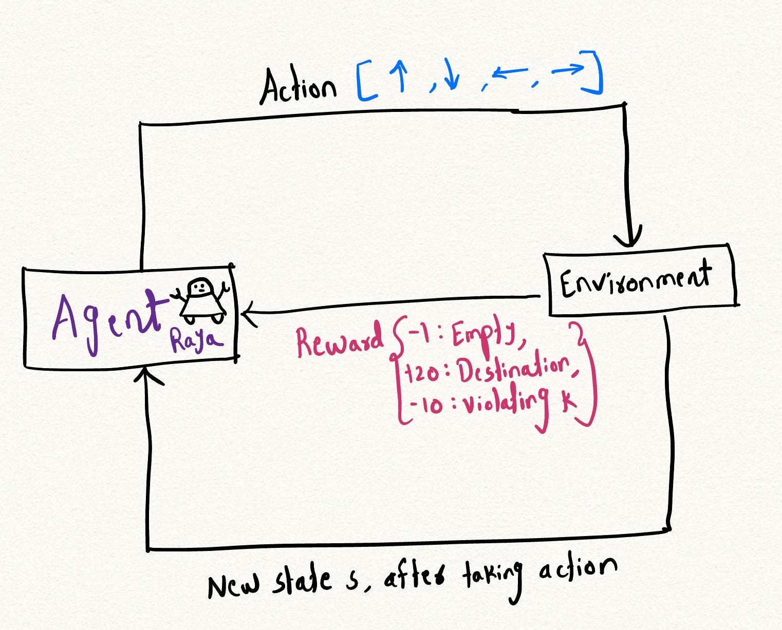
- Agent : An agent is a hypothetical entity that controls the course of action. You can imagine a hypothetical robot, say Agent Raya, that starts at a position and explores its environment. For instance, Raya has two possible options : position (0, 0) that goes right or to position (0, 1) that goes down, and both these positions have different rewards.
- Environment : The environment is the context in which our agent operates which is a two dimensional—a grid in this case.
- State : State represents current situation of the player. In our case, it gives current position of the player and the number of remaining violations.
- Reward System : reward is the score we get as a result of taking a certain action. In this case : -1 points for an empty cell, +20 points for reaching the destination and -10 points if we run out of the number of violations, k.
Through the process of iteration, we learn a optimal policy that allows us to find the best possible action at each time step that also maximized the total reward.
To be able to find the best policy, we used something called as a Q function. You can think of this function as a repository of all the exploration that your agent did so far. The agent then uses this historical information to make better decisions in the future that maximizes the reward.
Q function
Q(s, a) represents the expected cumulative reward an agent can achieve by taking action a in state s, while following policy π.
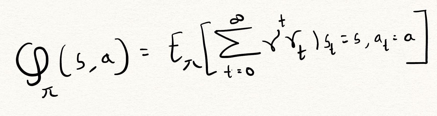
Where
- π : the policy adopted by the agent.
- s : the current state.
- a : the action taken by the agent in state s.
γ is the discount factor that balances exploration and exploitation. It determines how much priority the agent gives to immediate versus future rewards. A factor closer to 0 makes the agent focus on short-term rewards, while a factor closer to 1 makes it focus on long-term rewards.
The agent needs to balance exploiting known high-reward actions with exploring unknown actions that may potentially yield higher rewards. Using a discount factor between 0 and 1 helps prevent the agent from getting stuck in locally optimal policies.

Let's now jump into the code of how the whole thing works.
This is how we define an agent and the variables associated with it.
Reward Function : The reward function takes in the current state and returns the reward obtained for that state.
Bellman Equation :
How should we update the Q-table so that it has the best possible value for every position and action ? For an arbitrary number of iterations, the agent starts at position (0, 0, k), where k denotes the permitted number of violations. At each time step, the agent transitions to a new state by either exploring randomly or exploiting the learned Q-values to move greedily.
Upon arriving in a new state, we evaluate the immediate reward and update the Q-value for that state-action pair based on the Bellman equation. This allows us to iteratively improve the Q-function by incorporating new rewards into the historical, aggregated rewards for each state-action.
Here is the equation for bellman equation :

This is how the process of training looks like in code :
Build Path : For the path, we utilize the maximum Q value for each grid position to determine the optimal action to take at that position. The Q values essentially encode the best possible action to take at each location based on long-term rewards. For example, across all actions k at position (0,0), the maximum Q value corresponds to action "1", which represents moving right. By greedily choosing the action with the highest Q value at each step, we can construct an optimal path through the grid.
If you run the provided code, you will find it generates the path RBRBBB, which is indeed one of the shortest paths accounting for the obstacle.
Here is the link to the entire code in one file : _shortest_path_rl.py_
Conclusion
In real-world Reinforcement Learning scenarios, the environment the agent interacts with can be massive, with only sparse rewards. If you alter the configuration of the board by changing the 0s and 1s, this hardcoded Q-table approach would fail to generalize. Our goal is to train an agent that learns a general representation of grid-world configurations and can find optimal paths in new layouts. For the next post, I am going to replace the hardcoded Q-table values with a Deep Q Network (DQN). The DQN is a neural network that takes as input a state-action combination and the full grid layout and outputs a Q-value estimation. This DQN should allow the agent to find optimal paths even in new grid layouts it hasn't encountered during training.
Reach out to me on LinkedIn if you want to have a quick chat and want to connect : https://www.linkedin.com/in/pratikdaher/
