Support Vector Machine with Scikit-Learn: A Friendly Introduction
Among the available Machine Learning models, there exists one whose versatility makes it a must-have tool for every data scientist toolbox: Support Vector Machine (SVM).
SVM is a powerful and versatile algorithm, which, at its core, can delineate optimal hyperplanes in a high-dimensional space, effectively segregating the different classes of a dataset. But it doesn't stop here! Its effectiveness is not limited to classification tasks: SVM is well-suited even for regression and outlier detection tasks.
One feature makes the SVM approach particularly effective. Instead of processing the entire dataset, as KNN does, SVM strategically focuses only on the subset of data points located near the decision boundaries. These points are called support vectors, and the mathematics behind this unique idea will be simply explained in the upcoming sections.
By doing so, SVM Algorithm is computationally conservative and ideal for tasks involving medium or even medium-large datasets.
As I do in all my articles, I won't just explain the theoretical concepts, but I will also provide you with coding examples to familiarize yourself with the Scikit-Learn (sklearn) Python library.
Let's analyze Support Vector Machine (SVM) algorithms, and explore Machine Learning techniques, Python programming, and Data Science applications.
Linear SVM Classification
At its core, SVM classification resembles the elegant simplicity of Linear Algebra. Imagine a dataset in two-dimensional space, with two distinct classes to be separated. Linear SVM tries to separate the two classes with the best possible straight line.

What does it mean "best" in this context? SVM searches for the optimal separation line: a line that not only separates the classes, but does it with the maximum possible distance from the closest training instances of each classes. That distance is called margin. The data points that lay on the margin edge are the key element of the linear SVM classifier, and are called Support Vectors.

It is important to note that the separator is defined exclusively by the Support Vectors. As a consequence, adding more "off-the-street" training instances has no impact on the decision boundary. When more training instances that are not Support Vectors are added into the training set, the decision boundary doesn't move and those instances are "ignored". This feature is a great advantage of SVM, as it is not required to memorize the entire training set.
For an m-dimensional dataset, the separation line becomes a separation hyperplane, but the inspiring idea still holds.
Since the SVM model is based on distances, it is extremely sensitive to feature scales. For this reason it is always a good idea to normalize the features' values.
In Scikit-Learn we can instantiate a LinearSVC() object from the .svm module:
import pandas as pd
import sklearn
from sklearn import datasets

# Import the dataset
df_ = datasets.load_iris()
df = pd.DataFrame()
df['petal_length'] = df_['data'][:,2]
df['petal_width'] = df_['data'][:,3]
df['target'] = df_['target'] == 1

# Define train and test sets
X_train, X_test, y_train, y_test = sklearn.model_selection.train_test_split(df[['petal_length', 'petal_width']],
                                        df['target'],
                                        test_size=0.2,
                                        random_state=42)
# Normalize data
scaler = sklearn.preprocessing.StandardScaler()
X_train = scaler.fit_transform(X_train)

# Instantiate the classifier model
svm_classifier = sklearn.svm.LinearSVC()
# Fit the model with the training data
svm_classifier.fit(X_train, y_train)
# Predict new intances classes
y_predicted = svm_classifier.predict(scaler.transform(Xtest))
# Evaluate model's accuracy
accuracy = sklearn.metrics.accuracy_score(y_test, y_predicted)
print(accuracy)
The resulting accuracy is a mere 66%: not a remarkable result. In the next section, we will understand why the Linear Support Vector Machine classifier didn't perform better and what to do to cope with this.
Soft Margin Classification
As you can imagine, having a dataset whose classes can be perfercty separated by linear surfaces is a luxury. In a real-world scenario, it doesn't happen and data only needs one outlier to make it impossible for a Linear SVM to find a viable decision boundary.

As shown in the image above, in this case, there doesn't exist any line capable of separating the two classes.
To cope with real-world scenarios we need to introduce the Soft Margin Support Vector Machine Classification.
Unlike traditional Linear SVM (also called Hard Margin SVM), Soft Margin SVM doesn't require a rigid separation between the classes, allowing some elements of flexibility. By using a Soft Margin SVM, we acknowledge the existence of noisy data points and outliers.
More practically, we can specify an hyperparameter C which serves as a regularization parameter:
- setting
Cto a large value, we enforce a stricter margin, reducing misclassifications - setting
Cto a small value, we encourage a wider margin, allowing a greater number of misclassifications

There are two ways to implement the Soft Margin Linear SVM classifier in Scikit-Learn:
# Method 1
svm_classifier_soft = sklearn.svm.LinearSVC(C=10)
svm_classifier_soft.fit(X_train, y_train)

# Method 2
svm_classifier_soft = sklearn.svm.SVC(kernel='linear', C=10)
svm_classifier_soft.fit(X_train, y_train)
Running these lines of code for the same datasets, we obtain a slighter higher accuracy than the one we obtained for the Hard Margin LinearSVM. Although linear SVM classifiers are efficient and perform well in many scenarios, most datasets' classes are not linearly separable. In these cases, a linear decision boundary yields poor results.
Fortunately for us, SVM classifiers are not limited to linear decision boundaries. Thanks to the kernel trick, they can learn even the most complex separation shapes. The next section will focus on that.
Non-Linear SVM Classification
As I anticipated, many datasets are not linearly separable. Even if we account some flexibility, results obtained through a linear separation line are not optimal. To handle this issue, we can add more features, such as polynomial features. Adding new features will transform the original dataset into a higher-dimensional one, where it may be separated by a line or hyperplane.
Consider this simple example:

Data have only one feature and it is not separable by any straight line. If we add an artificial feature, computed as

we obtain the following dataset, which can be separated by a linear boundary:
However, adding polynomial features, like we did above, is not feasible for large and complex datasets. The resulting number of features would be too high.
Fortunately, there exists a technique called kernel trick that makes it possible even with high-degree polynomials. The mathematics behind the kernel trick is not complex, but as I want to focus on the practical implementation, I will leave this guide explaining it.
To implement a SVM classifier with a polynomial kernel in Python, we simply use the SVC() class and specify the type of kernel we intend to use and its degree:
# Instantiate the classifier object
SVM_classifier = sklearn.svm.SVC(kernel='poly', degree=5, C=10, coef0=1)
# Instantiate the scaler object
scaler = sklearn.preprocessing.StandardScaler()

# Normalize data
X_train = scaler.fit_transform(X_train)

# Train the classifier
SVM_classifier.fit(X_train, Y_train)
The coef0 hyperparameter acts as a regularization parameter, allowing to control how the model is influenced by high-degree polynomials.
Finding the correct balance between the degree, C andcoef0 hyperparameters is not a straightforward task. It is typically recommended to use a Grid Search approach to find some viable values, and later perform a finer manual search to tune them precisely.
Similarity Features: Gaussian Radial Basis Function
Polynomial kernels often work for a variety of Machine Learning problems, however, there exists a notable technique that often works even better: Similarity Features.
Instead of adding artificial polynomial features based on the original features' values, we place several landmarks in our high-dimensional feature space and measure the distance from them to each data point. These distance measures become the new model's features.
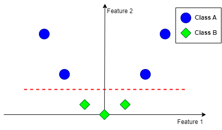
Consider a training set with two independent features that look like this:

By adding a certain number of landmarks in specific locations, we can create additional features computed as the distance from the data point to each landmark.

In this example, we can place two landmarks in those precise locations. The SVM classifier can then learn to predict as class A the instances close to the landmarks and as class B the ones far away from the landmarks.
Any distance measure can be used, however, it is proven to be convenient to implement the Gaussian Kernel function:

where:
- x is the vector containing the data point coordinates
- l is the vector containing the landmark coordinates
- gamma acts as a regularization hyperparameter
The question now is: "Where do I place the landmarks?". The most diffused approach is to place a landmark at each training example location. Having m training examples means creating m landmarks, and, as a consequence, it will result in m new features.
The downside of this approach is that for large training sets, we will end up with an equally large number of distance features.
In Scikit-Learn a SVM classifier with a Gaussian kernel is implemented as follows:
import pandas as pd
import sklearn
from sklearn import datasets

# Import the dataset
df_ = datasets.load_iris()
df = pd.DataFrame()
df['petal_length'] = df_['data'][:,2]
df['petal_width'] = df_['data'][:,3]
df['target'] = df_['target'] == 1

# Define train and test sets
X_train, X_test, y_train, y_test = sklearn.model_selection.train_test_split(df[['petal_length', 'petal_width']],
                                        df['target'],
                                        test_size=0.2,
                                        random_state=42)
# Normalize data
scaler = sklearn.preprocessing.StandardScaler()
X_train = scaler.fit_transform(X_train)

# Instantiate the classifier model
svm_gaussian_classifier = sklearn.svm.SVC(kernel='rbf', gamma=6, C=0.001)
# Fit the model with the training data
svm_gaussian_classifier.fit(X_train, y_train)
# Predict new intances classes
y_predicted = svm_gaussian_classifier.predict(scaler.transform(X_test))
# Evaluate model's accuracy
accuracy = sklearn.metrics.accuracy_score(y_test, y_predicted)
Conclusion
In this post, we detailed the theory of this versatile and powerful model, and we understood how easy it is to implement it in Python through the Scikit-Learn library.
I conclude this introductory guide by delineating the pros and cons of Support Vector Machine model.
Without any question, the strength of SVM coincide with its accuracy in high-dimensional spaces, making it ideal for data with numerous features, like images or genetic data. Additionally, I must remark SVM versatility: beyond classification, it seamlessly adapts to regression and anomaly detection tasks. Finally, on the pros side, I must point out its flexibility. SVM ability to handle non-linear relationships through different kernel functions, grants it a vast application spectrum.
As we all know the mantra "there is no free meal in Machine Learning", we must acknowledge SVM cons. First of all, SVM can easily be affected by noisy data, as we saw in the Linear SVM section. Scalability is also an Achilles heel for SVM: training large datasets with SVM can be computationally intensive and demanding.
As I reach the end of this guide, I need to point out that, despite having touched all the most relevant aspects of SVM, its field extends far beyond the insight provided here. For this reason, I recommend digging into the resources and references attached to this article.
If you liked this story, consider following me to be notified of my upcoming projects and articles!
Here are some of my past projects:
Social Network Analysis with NetworkX: A Gentle Introduction
Ensemble Learning with Scikit-Learn: A Friendly Introduction
Use Deep Learning to Generate Fantasy Names: Build a Language Model from Scratch
