The Biggest Weakness Of Boosting Trees
Introduction
I have been a Data Scientist for five years, and over those five years, I have had the opportunity to work on countless projects of various types. Like many Data Scientists, I began to develop a reflex when working with tabular datasets: "If it is tabular, feature engineering + a boosting algorithm will do the job!" and I wouldn't ask myself further questions.
Indeed, Boosting Algorithms have topped the state of the art for tabular data for so long that it became very difficult to question their supremacy.
In this article, we will dive into some interesting parts of the theory behind boosting algorithms and, in particular, their core component, the decision trees, and understand the scenarios in which you should be particularly careful when dealing with Boosting Algorithms facing Data Drift.
A brief discussion on data drifting through the prism of Linear Regression
Data drift, in its simplest definition, is the fact that the distribution of your data changes over time, which can impact your Machine Learning models.
For a long time, I believed that data drift was not a significant issue as long as the underlying relationship between the data remained similar, naively extrapolating my knowledge from linear regression to other model families.
The case of a change in the underlying relation
The case of an underlying relationship changing over time occurs when, for any given reason, the relationship between your features and your target changes over time.
For example, imagine a model that captures locally the price of real estate in a city. Among other factors, the price of an asset can be related to its geographic location. New construction (for example, a new train station, mall, or park) can affect the relationship that existed before between those features: the underlying relationship has changed.

If you trained a linear regression model considering only data before the new construction, your model might become completely inaccurate after a while when the effect of the new construction is reflected in the prices of the assets locally, and you would have to retrain a model.

In this case, it is easy to understand why: your model learned a relationship. The relationship has changed; hence, you need a new model to capture the new relationship.
In the example above, the relationship changed at one point in time, but in real life, the relationship can evolve continuously, and you might want to retrain also continuously to capture this modification over time.
The case of a global distribution drift
Let's now consider another situation which is more subtle.
This time, the relationship remains the same over time, but the change occurs in the distribution of values of our variable and our target. Staying with our real estate example: assume there is a linear relationship between the general inflation in a country and the real estate prices, and this relationship remains constant over time. The inflation is measured from a reference date and will grow over time, which will impact the prices of houses and apartments.
In this case, inflation is not bounded and will grow over time, even if the relationship between inflation and prices is not affected by time.

In the case of linear regression, this drift will have no impact on the model because the relationship between X and y has not changed.

While this type of drift might not seem like a significant issue due to the underlying relationship not changing, it becomes a huge problem when you use a model coming from the family of Decision Tree Models (like boosting trees), and we are going to explore this in the next section.
A real life example of distribution drift
In a recent Kaggle competition, competitors were asked to provide a model that could predict electricity production in Estonia based on several pieces of information including:
- Historical weather / forecast data
- The amount of solar panels installed over time
- Previous production (lagged by a few days)
A simple representation of the problem
For simplification, and for the sake of this article, I will consider a fairly simple model where:
- Solar production is proportional to installed capacity
- Solar production depends on the hour of the day due to solar radiance (with no production at night). We use a Gaussian distribution centered on 12 to model this behavior.
- Cloud coverage negatively impacts production. Random noise is added to the signal to model the cloud coverage impact.
Overall, the formula below can summarize our model:

With:
- y = Electricity production
- C = Cloud coverage
- K = Capacity installed, which grow over time
- S = Solar Radiance due to the hour of the day
This is a very simple model, but it will be good enough for the purpose of this article. Note that the formula is nonlinear.
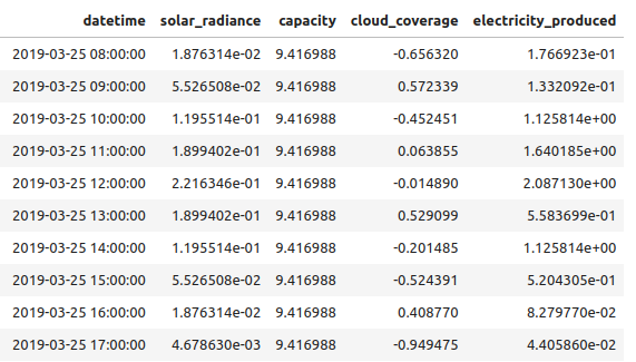
The code snippet provided below can help you generate a training set following the above formula:
import pandas as pd
import numpy as np

dates = pd.date_range(start='2019-01-01', end='2021-01-01', freq='H')

#capacity installed, growing by step over time
capas = np.ones(len(dates))
for i in [50,180,250,430,440,500,530,600]:
    capas[i*24:]=capas[i*24:]+np.random.random()*10

#Solar radiance impact, as a gaussian signal centered on 12hr
hours = np.arange(0, 24)
mean = 12
std_dev = 1.8
solar_radiance_list = (1/(std_dev * np.sqrt(2 * np.pi))) * np.exp(-0.5 * ((hours - mean) / std_dev) ** 2)

data = []
for i,date in enumerate(dates):
    cloud_coverage = np.random.random()*2-1
    hour = date.hour
    solar_radiance = solar_radiance_list[hour]
    electricity_produced = (np.clip(1-(cloud_coverage*1.3),0,1))*capas[i]*solar_radiance

    data.append(
        {
            "datetime":str(date),
            "solar_radiance":solar_radiance,
            "capacity":capas[i],
            "cloud_coverage":cloud_coverage,
            "electricity_produced":electricity_produced,
        }
    )
This will generate, zoomed in on a small window of time:
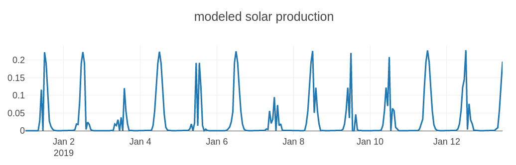
And, for the longer capacity increase trend:

In the figure above, bumps appear when a new solar plant is connected to the grid, providing more solar power.
The problem can be summarized as follows: "Given solar radiance, capacity, and cloud coverage, can we accurately estimate the electricity produced by the system?"
Building a model
The target we are trying to predict is highly nonlinear, but theoretically, we have all the relevant information to build a robust model.
C, K, and S are known, and I didn't add any extra noise. The data is tabular, so we can expect a boosting algorithm to perform extremely well on this task. I am using one year of data for training, which provides more than enough data points, and one year for testing, to accurately visualize what is about to happen.
X = df.drop(['electricity_produced','datetime'],axis=1)
y = df['electricity_produced']

train_split = 365*24
Xtrain, Xtest, ytrain, ytest = X.iloc[:train_split],X.iloc[train_split:], y.iloc[:train_split], y.iloc[train_split:]

lr = LGBMRegressor()
lr.fit(Xtrain,ytrain)
preds = lr.predict(Xtest)
And now, I am going to pause for a second. How well do you think the model is going to perform?
When I initially started on this, my first thoughts were that the model should perform very well. We have all the data we need, and the relationship we are looking to infer is invariant over time, theoretically protecting us from drifts.
But are we really protected?
Let's look at the predictions of the model against reality:
When we zoom in on the first dates of the test set, the predictions indeed seem perfect, and the model has correctly captured our formula.

However, when we examine more data points, this is what happens:

It's not so nice anymore. It looks like the model struggles to capture new variations in installed capacity.
Even if the relationship has not changed over time (I did not modify the formula I used), the model fails to capture the relationship for values outside of its training boundaries: this is a concrete example of failure due to feature drift!
When drift matters
In the example above, the distribution of capacity changes over time (it increases), but the relationship between the capacity and the target does not change (the formula remains the same).
For a long time, I used to believe that once a model has "learned" the underlying relationships between the data, it had learned them for good. However, this is not the case when dealing with decision trees (which are the foundation of boosting tree models).
To understand what is actually happening here, we need to take a closer look at how Decision Trees work.
How works Decision Trees
The basic behavior of a Decision Tree is to split the training data into areas for which the entropy of the target is minimized (i.e., zones where the target has more or less the same value).
In the case of a decision tree classifier, the model will consider as a reference the predominant class in the area, while a decision tree regressor will consider the average value of the area.
Let's revisit the simple example from part I and see how a decision tree regressor would build its prediction reference map.

And now you see the problem here: when X drifts toward higher values (greater than the boundary of the training set), all the points will be interpreted as part of the "reddish" reference area and will be predicted with the same value, regardless of the inner relationship between X and y.

A boosting algorithm is just a smart ensemble of decision trees
While boosting algorithms are highly efficient, they can ultimately be seen as a sophisticated form of bagging of decision trees. As such, they suffer from the same weaknesses, particularly this sensitivity to training boundaries.
This image represents the output of the prediction of a boosting model after training on the blue points.

Although I focused on regression here, the same behavior would occur with classification models.
How to solve this problem concretely?
Such data drifts actually occur everywhere in real datasets, and in this article, we have seen two examples where this phenomenon occurs.
Retraining models
One way to combat this data drift, the more obvious one, would be to adopt a strategy of constantly retraining your model, similar to what we would do if we suspected a change in the relationship over time. This method can adapt well to datasets for which the drift is slow relative to the amount of data available in a given period.
The main drawback is that, depending on your dataset and the amount of data needed to train a model, retraining could quickly become very expensive, especially if it needs to be done frequently.
Bounding your dataset with feature engineering
Ultimately, the problem of distribution drift, as presented here, comes from a feature going outside of the training bounding box. Sometimes, you can easily normalize your problem so that your features and target stay within fixed bounds.
For example, in the case of the solar farm mentioned earlier, we could recognize that both the target and the installed capacity are drifting, but that there is a simple relationship between them (thanks to field knowledge or data exploration).

Hence, we could build a normalized version of the target divided by the installed capacity.

In this new scenario, we would focus on predicting y_norm (bounded) with features like cloud coverage (bounded) and radiance (bounded). Then, we could determine y by simply multiplying our prediction by the installed capacity.

Normalizing the target with installed capacity removes the influence of the drift, allowing us to safely apply our boosting tree model.
Conclusion
In this article, we observed that boosting trees are very sensitive to distribution drifts due to their inherent nature as a "smart ensemble of decision trees," and this sensitivity persists even if the underlying relationship does not change.
The inspiration for this article came after noticing that many public notebooks for the electricity forecast competition were not considering any strategy to combat data drift. I, myself, had not considered distribution drifts until now unless I suspected a change in the underlying relationship in the data.
Delving deeper into the subject allowed me to truly understand the phenomenon at play here, and I hope this article also sheds light on something new for you. As data scientists, we must never forget that even the most powerful models have their weaknesses and that understanding the fundamentals is crucial to truly deliver high-quality work.
Thank you for reading!
