The Taylor Series, Explained

If you are angry at the Taylor series and surprised at its uselessness, as if its sole purpose of existence is to create tasks for us to solve, this post is probably for you.
Intro: Sequences and series
This section is here to refresh some basic knowledge. The first thing is the definition of series and sequences. A finite series is obtained by adding up the terms of a finite sequence. But in the context of real analysis, those finite series are usually left behind since without infinity, it doesn't make sense to talk about convergence, rates of convergence, etc., which is fundamental in real analysis.
In the case of an infinite series, there are infinitely many of those terms from an endless series. The sum up to any specified term is called a partial sum. [2]
The idea of a sequence is pretty straightforward, it's an ordered list of numbers that follow a particular pattern and looks like this: _a1, _a2, _a3, …_an. But it's useful to think about it as a function, this gives the formal definition of sequence:
A sequence is a function f: ℕ → ℝ, where ℕ is the set of non-negative integers (so 0 is included), and ℝ is the set of all the real numbers.
It would be a good idea to start from the following simple-looking sequence that will be revisited again and again:

we can see that this is a function that maps integers to real numbers:

but usually, it's preferred to denote this sequence as _{an}, since they are thought of as different types of objects than functions, i.e. a set of values. [3] Also, the notation _{an} resembles set notation. So (1.1) can be denoted as

Based on the definition of sequence, we can define partial sums mentioned a while ago as another sequence:
Given a sequence _{ak}, a new sequence can be defined by _{Sn} where _S_n=a₁+a₂+…+an. The sequence _{Sn} is called the sequence of partial sums of _{ak}.
The partial sums can be also written compactly as

Then
an infinite series is the limit of a particular sequence and that particular sequence is the sequence of the partial sum.
The infinite sequence is thus the following expression

The convergence of series
The example we choose here belongs to the geometric series, which is a series with the following form:

The coefficient in front of each item is the same constant k. And the partial sum of the first n items is (proof omitted because it's technical and doesn't offer much insight into our topic)

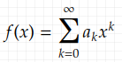
In addition, geometric series are special cases of power series which has the form

where c is the center of the power series. (The important concept of "center" will be revisited later.) We say that a series converges if _SN is finite when N approaches infinity, and diverges if _SN does not have a limit, i.e. the value of _SN "explodes" when N approaches infinity.
One of the reasons why example (1.1) is chosen as an introduction is that it's "simple", in the sense that the behavior of this type of series can be well classified:
- If |r|<1 then (2.1) converges.
- Otherwise (2.1) diverges.
Similarly for power series (2.3), exactly one of the following is true
- There is a unique positive real number R such that (2.3) converges for |r-c|
- The series converges only when r = c. In this case R = 0.
- (2.3) converges for all r∈ℝ. In this case R = ∞.
We call such R the radius of convergence of a power series. It is half of the length of the interval of convergence. This means that if the radius of convergence is R then the series centered around c converges if r lies in the following open interval:

"Open" in the previous sentence is stressed because how the series behaves on the endpoints is unknown and needs to be inspected ad hoc.
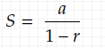
We can see that if we plug in r=1/2 and a=1 into (2.2), then we have the partial sum for (1.2):

and when n goes to infinity:

While evaluating the sum of infinitely many terms seems to be mission impossible, we did it and even got a constant!
When studying a series, two basic things to know are: (1) does it converge and (2) for what values does it converge? The next section will deal with this.
Determine the interval of convergence
Now we answer those questions. To determine whether a series converges or diverges, here are a lot of tests we can use depending on the series. The most important test here is the ratio test because it is also used to find the interval of convergence. And to keep this post from being too lengthy, we introduce only this one here: Let

be an infinite series. Set
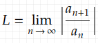
then there are three situations:
- If 0 ≤ L < 1, then (3.3) converges absolutely.
- If L > 1, then (3.3) diverges.
- If L = 1, the root says nothing.
So to find the interval of convergence of (2.3), we perform the ratio test on it, which gives

from what we have discussed before, we want to find the values of x for which (3.4) < 1.
This can be simply demonstrated by an example [6]: find the radius and interval of convergence of

performing the ratio test gives

thus the interval of convergence is given by solving 3|x| < 1, which is

and the radius of convergence is half the length of the interval of convergence, which is 1/3. We still don't know how the series would behave on the endpoints yet, so let's inspect it:
Plugging in -1/3 into (3.5) gives

which is a diverging p-series (proof omitted since it can be easily found). Therefore the endpoint -1/3 is not included.
Plugging in another endpoint 1/3 into (3.5) gives

which is an alternating p-series that converges (proof omitted here as well). Therefore, the endpoint 1/3 is included.
In conclusion, the interval of convergence of (3.5) is

Simple derivation of the Taylor series
More generally, from (2.2) we can deduce in the same way that _Sn is given by a closed form:
If you consider the ratio r as a variable and write it as a function

and this gives us a new insight that the function (4.1) can be expressed as the power series. Note that from here on we change the notations: r becomes x and the center c becomes _x0 since now the context switches to representing functions using series. And this raises an important question which brings us closer to the Taylor series:
How about other functions, can all the functions be expressed by means of power series?
The answer is almost yes. A lot of functions can be expressed this way, but not all of them. And even when a function has Taylor expansion at a point, the Taylor series can be useless and doesn't converge to the function.
From here on we are going to examine two theorems from [5] about representing functions using power series. Those two theorems will help us reveal the secret of the Taylor series.
The first one is the theorem on the transformation to a new center.
Let

be a power series with positive radius R. If _|x-x0| < R, then the function f(x) represented by this series can also be expanded in a power series:

in a neighborhood of _x0. Every coefficient _bn is represented by the absolute convergent series

which is a power series with the exact radius R. Furthermore, the radius _R1 of (4.3) is at least _R-|x0|.
We can see that (4.3) is acquired by shifting the center of the power series representing (4.2) to the right by _x0. According to this theorem, after shifting the center, the new series has different coefficients, which are described in (4.4). But the radius of convergence stays the same.
This theorem of center transformation can be proved by contradiction, it's somehow lengthy and we will omit it here. We will just show why (4.4) is what it is. Before we start, let's have a look at the binomial theorem which will be used to acquire (4.4):
Let n be a positive integer, and x and y be real numbers. The coefficient of x^k ∙ y^(n-k) in the kth term in the expension of (x+y)^n is equal to n choose k, which means

The trick is to rewrite (4.2) as

then we can simply apply the binomial theorem on (4.5) which gives us

where the series marked blue is just (4.4) starting from a different index. (The order of summation is swapped.)
The second theorem is about the differentiability property of functions represented by power series:
A function represented by a power series, say
is differentiable arbitrarily often at every interior point of its radius of convergence |r|
Using this theorem we can derivate (4.6) term-by-term, and shifting the index by 1 gives

Then we perform derivation again on (4.7) and this gives

which can be written as

because the binomial coefficient is defined as

so

doing this n times thus gives

pluging in x=0 we can directly get

which is going to be the coefficients of the Taylor series. Now we can plug (4.8) into (4.2) and get the following representation of f(x)

for more general cases not centered at 0 (4.3), f(x) is represented as

Here it is! (4.10) is the Taylor series or Taylor expansion (those terms are used interchangeably in this post). And (4.9) is known as the Maclaurin form of the Taylor series.
The meaning of "center"
We have talked a lot about the form of the Taylor series, but what does it mean that the series is "centered at a point" and what's the intuition behind this? This is essential for understanding how the Taylor series can be used to approximate functions but is left unexplained. So here we will have a look at this. The example used here for demonstrating the Taylor series at different centers is again (4.1):

Firstly we need to write (5.1) as a series centered at a different point, say 1/2, which means we need to find a new series with coefficient b_n such that

we have already seen before that simple substitution won't give us the series at a different center – all the coefficients need to be changed. And in this example, we can do it this way, i.e. transform (5.1) into a convenient form, for which we can directly write off the Taylor series:

To understand this better, here is a visualization of the first 5 orders of the Taylor series, we can see from the graph that they are two completely different series (the scripts can be found here):


Also, from this, we can intuitively understand what "locally" and "neighborhood" means: when the series moves further from the center, it is no longer close to the original function.
Note that when _x=x0, all the terms in the series, except the first that is f(x) (k=0), become 0 (for k=1, 2, 3, …). So, when x=x_0, the value is exactly f(x).
Another important fact that we need to keep in mind is that the radius and interval of convergence change after this shifting of the center. From the theorem on the transformation of the center, we know that the new radius would be at least

The error bound of the Taylor series
Let's have a look at Taylor's theorem, where the error bound (remainder) is mentioned: If function f:(a,b) → ℝ is n+1 times differentiable in an interval _(a, b), a_nd let a<

where

and ξ is any point between x and c (ξ can be x or c, but not necessarily), it's not a typo, if it was meant to be a typo "ξ" would be too extravagant. In (6.0), the last term, _Rn(x), is the error of the approximation of f(x).
Here is the proof to make it clear why the error has the same form as the (n+1)-th order derivative and why the argument of function f^(n+1) is ξ instead of c. The proof repeatedly uses the Rolle theorem which is a special case of the mean-value theorem:
To prove that the error bound of a Taylor series approximation is (6.1) we want to show that

where s and _x0 are any two distinct points on the aforementioned interval (a, b).
let's define the following auxiliary function (which is just the left-hand side of (6.2) minus the right-hand side of (6.2))

where k is a value that makes F(s) = 0. The target is to show that

Since _F(x0) = 0, the Rolle theorem implies that there is _x1 strictly between _x0 and s such that _F'(x1)=0. It's easy to see that _F'(x0)=0 as well, so we use the Rolle theorem again and it implies that there is _x2 strictly between _x0 and _x1 such that _F"(x2)=0. Continuing this argument we can get all the way to x_(n+1) between _x0 and _xn such that

also deriving (6.3) n+1 times gives

since polynomials with order less than n become 0 after being derivated more than n times. So combining (6.6) and (6.7) we have (6.4).
This tells us that the remainder of the Taylor series of order n has the same form of the n+1 th term. But the function argument is unknown, we just know that it's any point between x and _x0.
The definition of analytic functions
Another question that naturally arises at this point is: when does a function equal to its Taylor series? The simple answer is that at all the points x, where the remainder R_n goes to 0, as n approaches infinity. To be more practical, the following theorem gives a useful bound on R_n:
If

for all x in the interval _[x_0-d, x0+d] then the Taylor series converges to f on this interval and the remainder satisfies the inequality

for all x in _[x_0-d, x0+d].
And when a function is such, i.e. locally equals its Taylor series, it's analytic. The analyticity of a function has two equivalent definitions:
I. A function f is called analytic at a point _x0∈ℂ (ℂ is the set of all the complex numbers), if _f(x0) is differentiable for all points in some open set in ℂ. (Don't worry about ℂ too much, in this post we deal only with real numbers, but they are all complex numbers anyway.) And it's important to note that analyticity is always a property of a function on an open set (neighborhood around a point).
II. A function f is analytic at the point _x0 if its Taylor series centered at x_0 converges to f(x) for all x sufficiently close to _x0.
Those two definitions are equivalent, though doesn't appear so at first glance. The proof can usually be found in textbooks about complex analysis. (We omit it here.)
Another important fact is that analyticity implies differentiability but not vice versa. In another word
any function that is infinitely differentiable at a point x has a Taylor series at that point. But whether that Taylor series converges at any point around x is another issue.
A great pathological example to show this is the function around 0

the function is continuous and infinitely differentiable at point 0, but it's not analytic at point x=0 since all the derivatives of (7.2) are 0 at x=0. Therefore, as shown in the following graph, the Taylor series converges to the constant function f(x)=0 around point x=0, but not to (7.2).

A numerical example
A more practical problem we can use the Taylor series to solve is something like getting the approximate value of 8^(1/3), a numerical approximation. What we can do is view it as a point on the function x^(1/3) and calculate the Taylor series of this function centered at 8. [7]
Here we use the first three terms (order 2). Since we want to approximate the value of f(8.1), apparently we should set x = 8.1, and we know that 8^(1/3) = 2, so 2 is a very convenient neighbor point. This makes _x0 = 2, i.e. our Taylor series is centered at 2. Calculating the derivatives gives

and plugging in the values gives:

This evaluates to approximately 2.0082986111 (we keep up to the 10th decimal place). Then we calculate the remainder _R3:

plugging in the known values we get

and we want to find the upper bound of (8.2). Referring to the (8.1) we have calculated before, we can see that (8.2) is a monotonic increasing function on the interval [8, 8.1], therefore the upper bound should be

The awkward thing is that we need to evaluate 8.1^(1/3) again! But we know that 8.1^(1/3) is not very far away from 8^(1/3), which is 2. So in this case we can try to calculate the lower bound of the remainder _R3 which is

This is approximately 0.00000002411 (11th decimal place). If we use a calculator to compute 8^(1/3) directly, we get approximately 2.0082988502. The difference between our approximation and the value given by the calculator is about 0.00000002391 and we can see that 0.00000002391 < 0.00000002411. We got lucky here, __ the error is bounded by the remainder, in fact even the lower bound of the remainder.
Other use cases
Apart from approximating function values, we can also use the Taylor series to evaluate integral when the function to be integrated is awkward (just a layman's word for nonelementary functions), and evaluate differential equations. [6]
Last but not least, the Taylor series also plays an important role in discrete mathematics. The generating functions can be used to transform discrete problems into continuous ones. A concrete example of this is finding the moment generating function (MGF for short) for a probability mass/density function.
Conclusion
In this post, we briefly reviewed the basics like the definition of sequence and series and the convergence of series. Then we start from the motivation – representing functions using power series. Using the properties of those functions that can be represented using power series, we showed a simple derivation of the Taylor series. After the Taylor series is formulated, the concept of "analyticity" is brought up. At last a numerical example is shown to make it more intuitive about how the Taylor series can be used to approximate functions locally and to bound the errors.
References:
[1] Ribet, K. A. (2015). Undergraduate Texts in Mathematics. S. Axler (Ed.). Springer.
[2] Thompson, S. P., & Gardner, M. (2014). Calculus made easy. St. Martin's Press.
[3] Smits, T. (n.d.). Math 31 calculus and analytic geometry notes. University of California, Los Angeles. Retrieved August 24, 2024, from https://www.math.ucla.edu/~tsmits/31notes.pdf
[4] Hunter, J. K. (2014). An introduction to real analysis. Draft. Dept. of Mathematics, University of California at Davis. Available on the Web.
[5] Knopp, K. (1956). Infinite sequences and series. Courier Corporation.
[6] Stewart, J. (2007). Essential calculus: Early transcendentals. Brooks/Cole, a part of the Thomson Corporation.
[7] Brilliant.org. (n.d.). Taylor Series approximation. Brilliant. Retrieved September 2, 2024, from https://brilliant.org/wiki/taylor-series-approximation/
[8] MIT OpenCourseWare. (2010). Problem set 8 solutions: Single variable calculus (18.01SC). Massachusetts Institute of Technology. https://ocw.mit.edu/courses/18-01sc-single-variable-calculus-fall-2010/51bf782966d0896f0c183541e1c3cf22_MIT18_01SCF10_ex98sol.pdf
