Tiny Time Mixers (TTM): A Powerful Zero-Shot Forecasting Model by IBM

Author:Murphy | View: 21159 | Time: 2025-03-22 21:21:47

If you follow the latest research on LLMs, you will notice two main approaches:

First, researchers focus on building the largest models possible. Pretraining on next-word prediction is crucial for enhancing performance (and where the millions of dollars are spent!).

Second, researchers use techniques like quantization to create smaller and faster models – while maintaining strong general performance.

However, interesting things happen when smaller models outperform much larger ones in some tasks. For example, Llama 3–8B outperformed the larger Llama 2–70B on the MMLU task!

Tiny Time Mixers (Ttm)[1], introduced by IBM, follows the second approach. It's a lightweight model that outperforms larger SOTA models – including MOIRAI, on the M4 dataset. Plus, it's open source!

This article discusses:

The architecture and functionality of TTM.
The innovative features that make TTM exceptional.
Benchmark results comparing TTM with other models.

Let's get started!

I've launched AI Horizon Forecast, a newsletter focusing on time-series and innovative AI research. Subscribe here to broaden your horizons!

Enter Tiny Time Mixer (TTM)

TTM is a lightweight, MLP-based foundation TS model (≤1M parameters) that excels in zero-shot forecasting, even outperforming larger SOTA models.

Key characteristics of TTM:

Non-Transformer Architecture: TTM is extremely fast because there's no Attention mechanism – it only uses fully-connected NN layers.
TSMixer Foundation: TTM leverages TSMixer[2] (IBM's breakthrough time-series model) in its architecture.
Rich Inputs: Capable of multivariate forecasting, TTM accepts extra channels, exogenous variables, and known future inputs, enhancing its forecasting versatility.
Fast and Powerful: TTM was pretrained on 244M samples of the Monash dataset, using 6 A100 GPUs in less than 8 hours.
Superior Zero-Shot Forecasting: TTM is pretrained and can readily be used for zero-shot forecasting, surpassing larger SOTA models on unseen data.

Important Notes:

Note 1: There's a similar model by Google, also called TSMixer – which was published a few months later! Interestingly, Google's TSMixer is also an MLP-based model and achieves significant performance! In this article, we will only refer to IBM's TSMixer[2].

Note 2: IBM's TSMixer (where TTM is based on) applies softmax after a linear projection to calculate importance weights – which are then multiplied with hidden vectors to upscale or downscale each feature. The authors call this operation Gated Attention – but it's typically not a traditional multi-head attention with queries, keys, values and multiple heads. Therefore, neither TSMixer (or TTM that uses TSMixer) are characterized as Transformer-based models.

TTM Innovations

TTM introduces several groundbreaking features:

Multi-level modeling: TTM is first pretrained in a channel-independent way(univariate sequences) and uses cross-channel mixing during finetuning to learn multivariate dependencies.
Adaptive patching: Instead of using a single patch length, TTM learns various patch lengths across different layers. Since each time series performs optimally at a specific patch length, adaptive patches help the model generalize better across diverse data.
Resolution Prefix Tuning: Different frequencies (e.g. weekly, daily data) are challenging for foundation time-series models. TTM uses an extra embedding layer to encode time-series frequency – enabling the model to condition its predictions accurately based on the signal's frequency.

Tiny Time Mixers – Architecture

TSMixer is a precursor to TTM. TSMixer is a solid model, but it cannot be used as a foundation model or handle external variables.

TTM uses TSMixer as a building block – and by introducing new features, the authors created a non-Transformer model that generalizes on unseen data.

The architecture of TTM is shown in Figure 1. We'll describe both phases, pretraining(left) and finetuning(right):

**Figure 1:** *The top-level view of TTM architecture left(pretraining-phase), right(fine-tuning phase) (Source)*

Semantics: sl=context_size, fl=forecasting_length, c = number of channels (input features), c'= number of forecasting channels.

Note: If we have 5 input time-series, but 2 of them are known in the future (e.g _time_of_week, holiday_) then we have c=5 and c‘=5-2 = 3, because the two of them are known and don't need to be estimated.

Pretraining

During pretraining, the model is trained with univariate time-series only.
First, we normalize per individual time-series. The final outputs at the end are reverse-normalized (a standard practice).
Patching, a widely successful technique in time-series is also used here. Univariate sequences are split into n patches of size pl.
The TTM backbone module applies Adaptive patching and projects the patches from size p to hf. The TTM backbone is the heart of TTM and we'll explain it later in detail.
The TTM decoder has the same architecture as the TTM backbone – but it's much smaller, with 80% fewer parameters.
The Forecast linear head contains 1 fully-connected layer and produces the final forecasts (which are then reverse-normalized).
MSE loss is calculated over the forecast horizon fl.

Fine-Tuning

Here, the TTM backbone remains frozen and we only update the weights of the TTM decoder and Forecast linear head.
We can perform few-shot forecasting(train on only 5% of the train data) or full-shot forecasting (on the whole dataset).
We can use multivariate datasets in the fine-tuning phase. In that case, channel-mixing gets enabled in the TTM decoder.
Optionally, we can also activate the exogenous mixing block (shown in Figure 1) to model future known variables.

We just described the Multi-level modeling method of TTM: The model learns the temporal dynamics during pretraining in a channel-independent way, and inner-correlations between time series during finetuning.

TTM Backbone

The core component of TTM is the TTM Backbone – which enables Resolution Prefix Tuning and Adaptive Patching.

Let's zoom into this component to understand its functionality (displayed in Figure 2):

**Figure 2:** *Operations and tensor sizes of TTM backbone. **Resolution prefix** embeds granularity information in the model and **Adaptive Patching** applies dynamic patching across TTM levels.(Source)*

The embedding layer projects the patches from size pl to create the input embeddings of size hf.
Also, the Resolution Prefix Tuning module creates an embedding of size hf that represents the time-frequency/granularity – which is then concatenated with the input embedding (notice the n=n+1 operation in Figure 2).
The TTM block contains 3 sub-modules: the patch partition module, a vanilla TSMixer block, and a patch merging block:
The patch partition module increases the number of patches by K and decreases the patch length by K again. For example, in the first level, the input of size [c,n, hf] becomes [c, 4*n, hf//4].
The TSMixer block is applied to the transformed input andthe patch merging block reshapes the [c, 4*n, hf//4] input back to [c,n, hf].

Therefore, by using a different K at each level, channel-mixing is applied across different patches with different lengths. This is the Adaptive Patching process – which helps the model generalize on unseen data.

Exogenous Mixer

If we have future known variables, we can activate the Exogenous Mixer. This module is shown in Figure 3, and its position in the TTM architecture is shown in Figure 1:

The Exogenous Mixer block is straightforward: When the future values of time-series are known (y3 and y4 in Figure 3, green color), they are used to guide the predictions of the target variables (y1 and y2 in Figure 4, purple color).

TTM Training Details and Datasets

The authors created 5 TTM versions for different context sl and forecasting lengths fl. These are (512,96), (512,192), (512, 336), (512,720) and (96,24).

There's a configuration to use a shorter forecasting length for any of the above pretrained models

Regarding training, the authors used a subset of the Monash repository (244k samples) to pretrain the model and the Informer dataset to evaluate the finetuning performance. Also, the authors used another dataset to evaluate the efficacy of the exogenous mixer block and investigate how much the performance improves by adding known future variables.

You can find more about these datasets in the original paper. Below are the training hyperparameters for the (512,96) variant:

pl(patch_length) = 64
number of backbone levels = 6
number of TTM blocks per level = 2
batch_size = 3K
epochs = 20

For more details about the training and fine-tuning configurations, please refer to the original paper.

Evaluation Benchmarks

TTM vs SOTA models

Next, the authors evaluated both versions of TTM (Zero-shot and 5% Few-shot) against other SOTA models, including foundation models. The evaluation metric was MSE. The results are shown in Table 1:

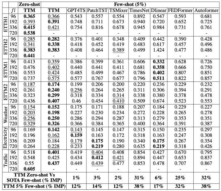
**Table 1:** *Comparing TTM with other SOTA models for various prediction lengths in terms of MSE. IMP stands for improvement. (Source)*

The results are quite impressive:

On average, Few-shot TTM surpassed all the other models. Even Zero-shot TTM was able to surpass some models! Remember, Zero-shot TTM produces forecasts without being trained on these data.

TTM also surpassed GPT4TS, a new foundation time-series model introduced last year.

Apart from the winning TTM, the next highest-ranking models are GPT4TS, PatchTST, and TSMixer – all of which utilize patching. Recent research in time-series forecasting has shown that patching is a highly beneficial technique.

TTM vs foundation models

The authors evaluate TTM individually against foundation models, notably GPT4TS and LLMTime:

LLMTime uses GPT-3 and LLaMa-2 with specific modifications tailored for time-series forecasting.
GPT4TS is a universal time-series model for many tasks (forecasting, classification, etc) and uses GPT-2 as a base model.

The comparison results are shown in Table 2 (LLMTime) and Table 3 (GPT4TS):

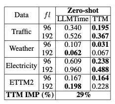
**Table 2:** Comparing Zero-Shot TTM against LLMTime, showing an average improvement of 29% over LLMTime. (Source)

**Table 3:** *Comparing 10% Few-Shot TTM with GPT4TS in terms of MSE. nx denotes n times average improvement (IMP) of MSE across benchmarked datasets. (Source)*

LLMTime was evaluated in a zero-shot forecasting scenario, while GPT4TS as a few-shot forecaster.

In both comparisons, TTM is the clear winner.
Additionally, TTM is much faster and requires significantly fewer resources. This is expected, as TTM does not utilize heavy Transformer computations like GPT4TS.

Effectiveness of Exogenous Variables

Modern real-world datasets use exogenous variables whenever possible – hence it makes sense to leverage them in a forecasting application.

The authors of TTM also investigated how TTM improves by using such variables (if applicable). Specifically, they compared Zero-Shot TTM, plain TTM, and TTM with channel-mixing (TTM-CM) that uses exogenous variables.

They also evaluated TSMixer and its channel-mixing variants. The results are shown in Table 4:

**Table 4:** *The impact of decoder mixing and exogenous variables in performance. (%IMP shows the percentage improvement of MSE) (Source)*

Again, the results are very interesting: First, TTM-CM ranks first, meaning that exogenous variables indeed help the model.

The TSMixer variants that use channel-mixing properties come in second place. Furthermore, Zero-Shot TTM performs the worst. It's clear that when auxiliary variables are present, they should be used to boost model performance.

Tiny Time Mixers In Practice

Check the AI Projects folder for extentive tutorials tutorials on the latest novel time-series models, including TTM.

We can download the weights of model versions 512–96 and 1024–96 on HuggingFace, and fine-tune it as follows:

import numpy as np
import pandas as pd
import matplotlib.pyplot as plt

from tsfm_public.models.tinytimemixer.utils import (
    count_parameters,
    plot_preds,
)

from tsfm_public.models.tinytimemixer import TinyTimeMixerForPrediction
from tsfm_public.toolkit.callbacks import TrackingCallback

zeroshot_model = TinyTimeMixerForPrediction.from_pretrained("ibm/TTM", revision='main')
finetune_forecast_model = TinyTimeMixerForPrediction.from_pretrained("ibm/TTM", revision='main', head_dropout=0.0,dropout=0.0,loss="mse")

Hence, we can use the familiar Trainer module from the transformers library to finetune TTM:

Note: Don't try to fine-tune TTM on a popular public dataset such as solar – TTM was pretrained on them. Check the original paper to find which datasets TTM has used for pretraining. Here, we fine-tuned on a private dataset, so we omitted some parts:

finetune_forecast_trainer = Trainer(
model=finetune_forecast_model,
args=finetune_forecast_args,
train_dataset=train_dataset,
eval_dataset=valid_dataset,
callbacks=[early_stopping_callback, tracking_callback],
optimizers=(optimizer, scheduler))

# Fine tune
finetune_forecast_trainer.train()

**Figure 4:** *Training and validation MSE losses of TTM (Image by author)*

predictions_test = finetune_forecast_trainer.predict(test_dataset)

And then plot the results after getting predictions on a private dataset:

**Figure 5:** *Plotting predictions for the 512–96 TTM variant (Image by author)*

Closing Remarks

Tiny Time Mixer (TTM) is a novel model that followed a different approach – and paves the way for smaller, but efficient models.

Specifically, TTM didn't use Attention and proved that we can still build a formidable TS foundation model.

The first time-series models with meta-learning capabilities that only used MLPs were N-BEATS and N-HITS. Let's see how this trend continues.

Recently, we have observed this trend with NLP models as well. We see Mamba(State Space) xLSTM (RNN-based) and Hyena (CNN-based) which are language models but not Transformers, achieving impressive results in numerous benchmarks.

Let's see how this approach unfolds for time-series models as well – after all, the research of foundation models is still new for time-series!

References

[1] Ekambaram et al., Tiny Time Mixers (TTMs): Fast Pre-trained Models for Enhanced Zero/Few-Shot Forecasting of Multivariate Time Series (April 2024)
[2] Ekambaram et al., TSMixer: Lightweight MLP-Mixer Model for Multivariate Time Series Forecasting (June 2023)