Unlock the Secrets of Causal Inference with a Master Class in Directed Acyclic Graphs

Objective
Having spent a lot of time researching causal inference I began to realise that I did not have a full grasp of Directed Acyclic Graphs (DAGs) and that this was hampering my efforts to develop my understanding to a point where I could apply it in order to solve real-world problems.
This objective of this article is to document my learning journey and to share everything you need to know about DAGs in order to take your understanding of Causal Inference to the next level.
Background
I would like to start by proposing a definition for Causal Inference –
Causal inference is the process of reasoning and the application of conclusions drawn from cause-and-effect relationships between variables while taking into account potential confounding factors and biases.
That is quite a mouthful, but it does encapsulate the key points –
- It is the study of cause-and-effect.
- The point is to draw conclusions that can be applied to solve real-world problems.
- Any bias or "confounding" must be taken account of and compensated for.
Moving beyond the definition, there is an age old saying that "correlation does not imply causation" which leads to the question "so what does then?"
It turns out that causation cannot be inferred or calculated from a set of data in isolation. That data needs to be extended and supplemented with additional information that can propose, visualise and represent the causal relationships and one common approach to the is to use a "Directed Acyclic Graph".
A Simple DAG
At the most basic level DAGs are very simple indeed. The example below is representing the proposed relationship between taking a drug "D" and recovery "R" and the arrow is stating that taking the drug has a causal effect on recovery …

This DAG illustrates two of the key terms – "treatment" and "outcome".
- "treatment" (drug in this example) refers to the action or intervention being studied or manipulated to determine its effect on the outcome.
- "outcome" (recovery in this example) refers to the variable being measured to determine the effect of the treatment.
In traditional machine learning terms, the treatment is the independent variable(s) and the outcome the dependent variable.
When I first studied DAGs I was confused by the terminology as "treatment" and "outcome" are typically medical terms and I wondered if DAGs and causal inference were limited to the medical domain. This is not the case; causal inference can be applied to any set of variables in any domain and I suspect the medical-sounding terminology has been borrowed because drug and treatment trials have a significant overlap with causal inference.
A DAG with a "Confounder"

This example adds another factor – "G" or gender. The arrows show that gender (G) has a causal affect on both the drug (D) and on recovery (R). The explanation for this is as follows –
- More males than females decide to take the drug so "Gender" causes "Drug".
- Females have a better natural recovery rate than males so "Gender" causes "Recovery".
This complicates things significantly. The objective is to establish the true effect of taking the drug on recovery but gender is affecting both so simply observing how many people in the trial took the drug and recovered does not provide an accurate answer.
This mixing effect is called "confounding" and a variable that causes this effect is a "confounder" which must be "de-confounded" to establish the true efficacy of the drug …
Randomized Control Trials, Stratification, Conditioning, Controlling and Covariates
In order to calculate the true effect of D on R we need to isolate and remove the effect of G. There are several approaches that can be applied including the following …
Randomized Control Trials
If this was a future trial that was being planned, one tried-and-tested approach would be to create a "Randomized Control Trial" (RCT). This would involve randomly assigning the drug trial subjects into a test group that receives the drug and a control group that received a placebo. (Note: it is important not to tell the subjects which group they have been allocated to).
It is now impossible for gender to be causing or influencing who takes the drug because subjects are assigned randomly. This effectively "rubs out" the causal relationship between "G" and "D" which means that any observed effect of the drug on recovery will now be independent of the confounding effect –

However, if the study is based on a historical trial where the data has already been recorded it is too late to randomly assign the test and control groups and an RCT cannot be used.
Another big challenge with RCTs is that if the "treatment" being studied is smoking or obesity it is not possible to randomly assign into a smoking group or obese group so clearly there are moral and ethical boundaries that limit the applicability of RCTs.
Fortunately, there are other approaches that can be applied to historical, observational data to mitigate these challenges including "stratification" …
Stratification
In our example, if the subjects were 60% male and 40% female the effect of the drug "D" on recovery "R" can be isolated and calculated as follows –
- Calculate the recovery for males and multiply by 0.6 (as 60% are males).
- Calculate the recovery for females and multiply by 0.4 (as 40% are females).
- Add the two numbers together and this gives the effect of the drug on recovery independent from the impact of gender.
Unfortunately, if there are a large number of variables the stratification could become very complicated. For example, if there are 10 variables each with 10 possible values, we would already be up to 100 strata and if one or more of the variables were continuous the permutations would soon become overwhelming.
Conditioning
Using causal inference techniques it is possible to simulate the affect of a real-world Randomized Control Trial on historical and observational data.
This sounds like magic but it uses sound mathematical techniques that have been established, defined and described over many years by experts including Judea Pearl who has published his findings in academic journals and books including the following –
- The Book of Why
- Causal Inference in Statistics
This "simulation" of RCTs is achieved by applying something called backfoor adjustment to condition on all the confounders i.e. the variables that affect both the treatment and the outcome.
Here is the backdoor adjustment formula for a single treatment variable (X) on a single outcome variable (Y) with a single confounder (Z) –

The key takeaway is that the left hand side is describing an "intervention", for example "assign everyone to take the drug" (do(X)) which is re-written on the right hand side and expressed in terms of purely observational data.
A detailed explanation of the maths is beyond the scope of this article but if you would like to see a fully worked example, check this link out …
Unlock the Power of Causal Inference : A Data Scientist's Guide to Understanding Backdoor…
Controlling
Controlling is a statistical technique that refers to holding the value of a variable constant that might otherwise adversely affect the outcome of a trial.
For example, in a trial that is investigating the effect of Vitamin D on alertness the designers of the trial might decide to give all participants specific instructions about their diet, when they eat, caffeine intake, screen time, exercise and alcohol intake in an attempt to isolate the true effect.
There seems to be some healthy disagreement in the literature at this point. Statisticians often seem to control for everything they can, even in a Randomized Control Trial.
Proponents of causal inference in general and Judea Pearl in particular seem to advocate only controlling (or conditioning) on those variables that are specifically confounding the effect of the treatment on the outcome.
I do share Pearl's view that controlling for everything in a trial may not be necessary and may even have unintended negative consequences on the results. My reasoning is that in a Randomized Control Trial any external factors like caffeine intake etc. should average out within and across the groups because of the random selection of the participants and also how do we know for sure that the participants followed the instructions?
Also, the theory of Causal Inference does make a strong case for identifying an optimum set of variables to condition on and to limit the adjustments accordingly (more on this later).
Covariates
One definition of covariates are variables that affect a response variable but are not of interest in a study. Consider the following DAG …

H represents the hours of studying and is the treatment and E represents the exam score (the outcome) which are the only variables of interest.
However, a domain expert points out that prior student ability also affects the exam score and although it is of not interest to the study they introduce it to the model.
In this case G satisfies the definition of a covariate.
My personal observation is that covariates appear to be a concept used in statistical and observational analyses, and hence favoured by statisticians and that proponents of causal inference may be inclined to say that unless G is a confounder of H and E it does not need to be introduced into the model.
Note that I have included an explanation of covariates for completeness as they are often mentioned in the literature and it is important to be able to understand the points being made whilst appreciating the difference between covariate and confounders.
Recap
At this point we have defined causal inference, explored the purpose of DAGs and explained confounders, RCTs, stratification, conditioning and controlling.
RCTs, stratification and controlling are all statistical technqiues related to real-world trials.
Conditioning is a causal inference technique that can be applied to historical, obervational data to draw conclusions about the affect of a treatment on an outcome even where the participants of the original survey were not selected at random.
This instantly opens up a world of opportunity because there are lots of historical, observational datasets that can now be explored for cause-and-effect and this is just one of the many benefits of causal inference and directed acyclic graphs.
Armed with this understanding and terminology we are now ready to explore and the more complex aspects of DAGs which are often not explained clearly in the available books and online articles …
Paths
Paths are a difficult subject to master because the concepts and techniques are all inter-related making the order of learning difficult. In the sections below I present paths at a high level, then delve into the patterns of forks, chains and colliders.
This leads into conditioning, blocking and unblocking which only make sense when the topic of paths is completed by learning about how to condition an entire DAG to remove the effect of confounding and draw casual conclusions.
Let's start by considering the following Directed Acyclic Graph …
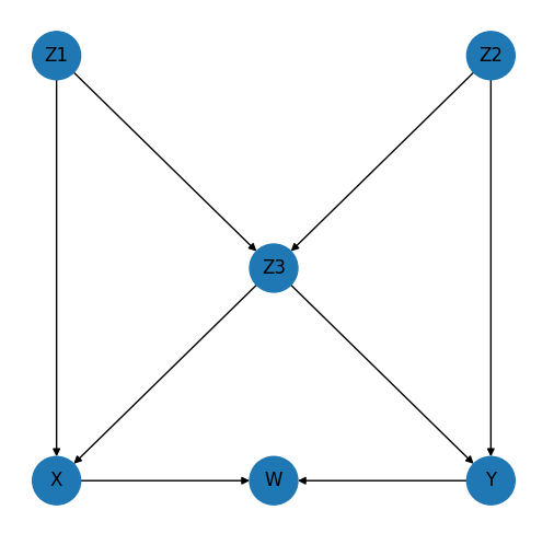
This is more complicated that the drug, gender, recovery example but quite staright-forward once the key concept of paths has been unpacked. I have not managed to find a definitive definition of "path" in the literature, so here is my definition …
A path is a sequence of causal links connecting the treatment and the outcome in a causal diagram.
In the above DAG therefore, a single path is
