Unlocking the Power of Interaction Terms in Linear Regression

Author:Murphy | View: 22230 | Time: 2025-03-23 18:34:43

Linear Regression is a powerful statistical tool used to model the relationship between a dependent variable and one or more independent variables (features). An important, and often forgotten, concept in regression analysis is that of interaction terms. In short, interaction terms enable us to examine whether the relationship between the target and the independent variable changes depending on the value of another independent variable.

Interaction terms are a crucial component of regression analysis, and understanding how they work can help practitioners better train models and interpret their data. Despite their importance, interaction terms can be difficult to understand.

In this article, we will provide an intuitive explanation of interaction terms in the context of linear regression.

What are interaction terms in regression models?

First, let's consider the simpler case, that is, a linear model without interaction terms. Such a model assumes that the effect of each feature or predictor on the dependent variable (target) is independent of other predictors in the model.

The following equation describes such a model specification with two features:

In order to make the explanation easier to understand, let's use an example. Imagine we are interested in modeling the price of real estate properties (y) using two features: their size (X1) and a boolean flag indicating whether the apartment is located in the city center (X2). β0 is the intercept, β1 and β2 are coefficients of the linear model and ε is the error term (unexplained by the model).

After gathering data and estimating a linear regression model, we obtain the following coefficients:

Knowing the estimated coefficients and that X2 is a boolean feature, we can write out the two possible scenarios depending on the value of X2.

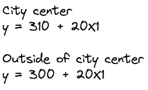
How to interpret those? While this might not make a lot of sense in the context of real estate, we can say that a 0 square meter apartment in the city center costs 310 (the value of the intercept) and each square meter of additional space increases the price by 20. In the other case, the only difference is that the intercept is smaller by 10 units. The following plot illustrates the two best fit lines.

*Regression lines for properties in the city center and outside of it*

As we can see, the lines are parallel and they have the same slope – the coefficient by X1, which is the same in both scenarios.

Interaction terms represent joint effects

At this point you might argue that an additional square meter in an apartment in the city center costs more than an additional square meter in an apartment on the outskirts. In other words, there might be a joint effect of these two features on the price of real estate.

So we believe that not only the intercept should be different between the two scenarios, but also the slope of the lines. How to do that? That is exactly when the interaction terms come into play. They make the model's specification more flexible and allow us to account for such patterns.

An interaction term is effectively a multiplication of the two features that we believe have a joint effect on the target. The following equation presents the model's new specification:

Again, let's assume we have estimated our model and we know the coefficients. For simplicity, we have kept the same values as in the previous example. Bear in mind that in a real-life scenario, they would most likely differ.

Once we write out the two scenarios for X2 (city center or not), we can immediately see that the slope (coefficient by X1) of the two lines is different. As we hypothesized, an additional square meter of space in the city center is now more expensive than in the suburbs.

Interpreting the coefficients with interaction terms

Adding interaction terms to a model changes the interpretation of all the coefficients. Without an interaction term, we interpret the coefficients as the unique effect of a predictor on the dependent variable.

So in our case, we could say that β1 was the unique effect of the size of an apartment on its price. However, with an interaction term the effect of the apartment's size is different for different values of X2. In other words, the unique effect of apartment size on its price is no longer limited to β1.

To better understand what each coefficient represents, let's have one more look at the raw specification of a linear model with interaction terms. Just as a reminder, X2 is a boolean feature indicating whether a particular apartment is in the city center or not.

Now, we can interpret each of the coefficients in the following way:

β0 – the intercept for the apartments outside of the city center (or whichever group that had a 0 value for the boolean feature X2),
β1 – the slope (effect of price) for apartments outside of the city center,
β2 – the difference in the intercept between the two groups,
β3 – the difference in slopes between apartments in the city center and outside of it.

For example, let's assume that we are testing a hypothesis that there is an equal impact of the size of an apartment on its price, regardless of whether the apartment is in the city center or not. Then, we would estimate the linear regression with the interaction term and check whether β3 is significantly different from 0.

Some additional notes on the interaction terms:

We have presented two-way interaction terms, however, higher-order interactions (for example, of 3 features) are also possible.
In our example, we showed an interaction of a numerical feature (size of the apartment) with a boolean one (is the apartment in the city center or not). However, we can create interaction terms of two numerical features as well. For example, we might create an interaction term of the size of the apartment with the number of rooms. Please refer to the sources mentioned in the References section for more details on that topic.
It might be the case that the interaction term is statistically significant, but the main effects are not. Then we should follow the hierarchical principle stating that if we include an interaction term in the model, we should also include the main effects, even if their impacts are not statistically significant.

Hands-on example in Python

After all the theoretical introduction, let's see how to add interaction terms to a linear regression model in Python. As always, we start by importing the required libraries.

import numpy as np
import pandas as pd

import statsmodels.api as sm
import statsmodels.formula.api as smf

# plotting
import seaborn as sns 
import matplotlib.pyplot as plt

# settings
plt.style.use("seaborn-v0_8")
sns.set_palette("colorblind")
plt.rcParams["figure.figsize"] = (16, 8)
%config InlineBackend.figure_format = 'retina'

In our example, we will estimate linear models using the statsmodels library. For the dataset, we will use the mtcars dataset. I am quite sure that if you have ever worked with R, you will be already familiar with this dataset. First, we load the dataset:

mtcars = sm.datasets.get_rdataset("mtcars", "datasets", cache=True)
print(mtcars.__doc__)

Executing the snippet prints a comprehensive description of the dataset. We only show the relevant parts – an overall description and the definition of the columns:

   ====== ===============
   mtcars R Documentation
   ====== ===============

   The data was extracted from the 1974 *Motor Trend* US magazine, and
   comprises fuel consumption and 10 aspects of automobile design and
   performance for 32 automobiles (1973–74 models).

   A data frame with 32 observations on 11 (numeric) variables.

   ===== ==== ========================================
   [, 1] mpg  Miles/(US) gallon
   [, 2] cyl  Number of cylinders
   [, 3] disp Displacement (cu.in.)
   [, 4] hp   Gross horsepower
   [, 5] drat Rear axle ratio
   [, 6] wt   Weight (1000 lbs)
   [, 7] qsec 1/4 mile time
   [, 8] vs   Engine (0 = V-shaped, 1 = straight)
   [, 9] am   Transmission (0 = automatic, 1 = manual)
   [,10] gear Number of forward gears
   [,11] carb Number of carburetors
   ===== ==== ========================================

Then, we extract the actual dataset from the loaded object:

df = mtcars.data
df.head()

For our example, let's assume that we want to investigate the relationship between the miles per gallon (mpg) and two features: weight (wt, continuous) and type of transmission (am, boolean).

First, we plot the data to get some initial insights.

sns.lmplot(x="wt", y="mpg", hue="am", data=df, fit_reg=False)
plt.ylabel("Miles per Gallon")
plt.xlabel("Vehicle Weight");

*Scatterplot of miles per gallon vs. vehicle weight, color per transmission type*

Just by eyeballing the plot, we can see that the regression lines for the two categories of the am variable will be quite different. For comparison's sake, we start off with a model without interaction terms.

model_1 = smf.ols(formula="mpg ~ wt + am", data=df).fit()
model_1.summary()

The following tables show the results of fitting a linear regression without the interaction term.

From the summary table, we can see that the coefficient by the am feature is not statistically significant. Using the interpretation of the coefficients we have already learned, we can plot the best fit lines for both classes of the am feature.

X = np.linspace(1, 6, num=20)
sns.lmplot(x="wt", y="mpg", hue="am", data=df, fit_reg=False)
plt.title("Best fit lines for from the model without interactions")
plt.ylabel("Miles per Gallon")
plt.xlabel("Vehicle Weight")
plt.plot(X, 37.3216 - 5.3528 * X, "blue")
plt.plot(X, (37.3216 - 0.0236) - 5.3528 * X, "orange");

*Best-fit lines for both types of transmission*

As the coefficient by the am feature is basically zero, the lines are almost overlapping.

Then, we follow up with a second model, this time with an interaction term between the two features. Below we show how to add an interaction term as an additional input in the statsmodels formula.

model_2 = smf.ols(formula="mpg ~ wt + am + wt:am", data=df).fit()
model_2.summary()

The following summary tables show the results of fitting a linear regression with the interaction term.

Two conclusions we can quickly draw from the summary table:

all of the coefficients, including the interaction term, are statistically significant.
by inspecting the R2 (and its adjusted variant, as we have a different number of features in the models), we can state that the model with the interaction term results in a better fit.

Similarly to the previous case, let's plot the best fit lines.

X = np.linspace(1, 6, num=20)
sns.lmplot(x="wt", y="mpg", hue="am", data=df, fit_reg=False)
plt.title("Best fit lines for from the model with interactions")
plt.ylabel("Miles per Gallon")
plt.xlabel("Vehicle Weight")
plt.plot(X, 31.4161 - 3.7859 * X, "blue")
plt.plot(X, (31.4161 + 14.8784) + (-3.7859 - 5.2984) * X, "orange");

*Best fit lines for both types of transmission, including interaction terms*

We can immediately see the difference in the fitted lines (both in terms of the intercept and the slope) for cars with automatic and manual transmissions.

Bonus: We can also add interaction terms using scikit-learn‘s PolynomialFeatures. The transformer offers not only the possibility to add interaction terms of arbitrary order, but it also creates polynomial features (for example, squared values of the available features). For more information, please refer to the documentation.

Wrapping up

When working with interaction terms in linear regression, there are a few things to remember:

Interaction terms allow us to examine whether the relationship between the target and a feature changes depending on the value of another feature.
We add interaction terms as a multiplication of the original features. By adding these new variables to the regression model, we can measure the effects of the interaction between them and the target. It is crucial to interpret the coefficients of the interaction terms carefully in order to understand the direction and the strength of the relationship.
By using interaction terms we can make the specification of a linear model more flexible (different slopes for different lines), which can result in a better fit to the data and better predictive performance.

You can find the code used in this post in my GitHub repo. As always, any constructive feedback is more than welcome. You can reach out to me on Twitter or in the comments.

Liked the article? Become a Medium member to continue learning by reading without limits. If you use this link to become a member, you will support me at no extra cost to you. Thanks in advance and see you around!

You might also be interested in one of the following:

A Comprehensive Overview of Regression Evaluation Metrics

Interpreting the coefficients of linear regression

One thing you might not have known about linear regression

The Minimalist's Guide to Experiment Tracking with DVC

References

- https://rinterested.github.io/statistics/lm_interactions_output_interpretation.html
- https://janhove.github.io/analysis/2017/06/26/continuous-interactions
- https://ademos.people.uic.edu/Chapter13.html
- https://joelcarlson.github.io/2016/05/10/Exploring-Interactions/
- Henderson and Velleman (1981), Building multiple regression models interactively. Biometrics, 37, 391–411.
- the
mtcarsdataset in R is part of the base R distribution and is released under the GNU General Public License (GPL)
All images, unless noted otherwise, are by the author.
Originally published at NVIDIA's developer blog on April 26th, 2023