Vectorisation What is it and how does it work?

This is the 2nd iteration of this article. After finishing the 1st iteration, I left it to stew and edit as the headlines didn't look good – a 13 min ramble about vectorisation with some loose links to database theory and historical trends.
While waiting to re-draft, I came across several performance comparisons of the new much hyped pandas 2.0 release – especially comparing it to Polars. At this point I must come clean – Pandas is Ground Zero for me and I'm yet to even pip install Polars for testing. I'm always hesitant to swap out a well known and supported package for anything new or in vogue until either:
- the existing tool is starting to fail (I'm not using large enough data post SQL-aggregation)
- there is some other clear compelling evidence for stomaching the adoption
However the relatively below par performance of the new Pandas 2.0 release did have me wondering – if Polars is so fast for in-memory operation, how is it achieving this?
The Polars author wrote my original article (but better)
Vectorisation. Polars is fast because the original author designed the whole thing to be about vectorisation. In this ‘hello world' post from Polars author Ritchie Vink he explains using a combination of clear concise sentences and simple visuals how Polars achieves what it achieves – because it is not just built with ideas of vectorisation in mind, but built completely around those principles.
The aim for the rest of this article isn't necessarily to rehash what has been said there, but instead to work back through some ideas and historical context to shed light on how we have come to column (or array) based computing being more ‘mainstream' and how that has started to perforate the modern day Data Science tool kit in python.
"I don't care what your fancy data structure is but I know that an array will beat it"
The above is from this talk by Scott Meyers where he attributes the above quote to the CTO of an algorithmic trading company championing an array. It's also eluded to in the Polars article but the idea is the same – when it comes to the actual practicalities, sometimes you need to chuck your basic time complexity analysis out the window because an O(n) algorithm can trump an O(1) algorithm.
I come from a non computer science background, but the wealth of material that universities (particularly American) make available online means I've been able to take some of the basic ‘Algorithms' and ‘Data Structures' courses. From what I can see, the joint aim could be (probably badly) summarised as:
- use logic to come up with a process that involves the least amount of steps (algorithms)
- organise your data to enable the selection of an algorithm with minimum steps (data structures)
The importance of understanding the core concepts of both is underscored by the legions of companies out there barraging their hopefuls with reams of Leetcode questions on Dynamic Programming or Binary Search Trees or any other generally day-to-day irrelevant topic. One such example is usually this – when it comes to looking stuff up use a hash map rather than an array. This is because:
- a hash map is O(1) to lookup
- an (unsorted) array is O(n) as you potentially need to traverse the whole thing
Why doesn't the above always hold? Because the statement "an O(1) algorithm is faster than an O(n) algorithm" is incomplete. The true statement should be more like "an O(1) algorithm is faster than an O(n) algorithm, conditional on the same starting point".
Driving a Ferrari in New York
Modern day CPUs have been described as similar to ‘driving a Ferrari in New York'. Needless to say the analogy has clearly come from a computer scientist who believes the only reason to drive a car is to get from A to B, but the point remains. Why do you need such a fast car if all you'll be doing is continuously stopping and starting (although stopping and starting really really fast)?
Substitute ‘car' for ‘processor' and we are looking at modern day CPUs. This has come about due to the relative speed improvements that have been and are continuing to be made (although at a much slower rate these days) in processor speeds vs memory speeds. This is illustrated beautifully in this C++ orientated talk by Herb Sutter (start at 12:00 for around 20mins if you want to just strip the overview) and the below chart shows it well:
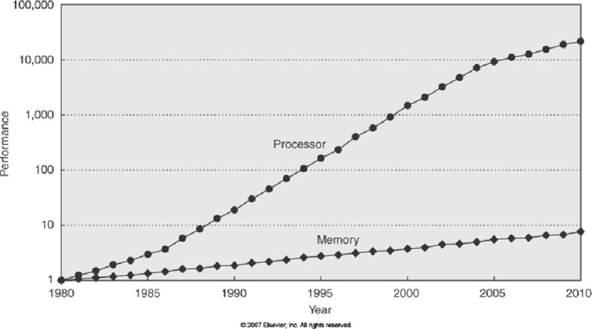
In simple terms we have a "Moore's Law induced" widening gap between how fast our processor can operate on stuff and how fast we can get that stuff to our processor. There's no need to have such a fast processor if it's sitting idle most of the time waiting for new data to operate on.
How do we circumvent this? Caching, caching and more caching
Below is the standard image that many people have of a computer's architecture (skip to 22:30 of Herb Sutter's talk for a comedic example of this):

In other words – we have:
- our CPU that does stuff
- our memory (or RAM) that is ‘quick' to access
- our disk which is slow to access
Now as the above graph showed, memory might be fast relative to retrieving data form disk – but retrieval certainly isn't fast relative to the data we can process with our current quantity and speed of processors. To solve this, hardware developers decided to put memory onto the CPU (or ‘die'). These are known as caches and there are several per each processing core. Each core consists of:
- an L1 cache: this is the fastest and is split into an instruction cache (storing the instructions that your code boils down to) and a data cache (stores variables that you are operating on)
- an L2 cache: larger than L1 but slower
and then all cores on a machine share an L3 cache – again larger than both L1 and L2 but slower again.
The below image, based on a blown up photo from an Intel white paper (The Basics of Intel Architecture (v.1, Jan. 2014)), shows how a 4 core CPU is laid out for Intel's i7 processor – L1 and L2 caches are within each ‘Core' section:

But the same applies for more up to date PCs. I'm writing this on a Macbook Air M2 and a quick lookup on Wikipedia indicates that the M2 chips contain L1, L2 and a shared ‘last level cache' (L3).
So how much faster is retrieving data from cache than memory?
For this – a picture is worth a thousand words – or more specifically, an animation. The following link from gaming software optimisation company Overbyte shows just how drastic the relative performance is: http://www.overbyte.com.au/misc/Lesson3/CacheFun.html.
Speeds vary between machines but – measuring time in the standard ‘clock cycle' unit we have roughly:
- L1: ~1–3x clock cycles
- L2: ~10x clock cycles
- L3: ~40x clock cycles
- Main memory: ~100–300x clock cycles
In other words: if our data is in L1 memory our computer will process it between 30–300x faster than if we fetch it from main memory. Main memory being RAM, not disk. When your CPU can't find the data in the L1 cache, it searches L2, then L3 and then it goes to main memory with each of these failed searches labelled a ‘cache miss'. The fewer cache misses you have, the faster your code.
So how do I get my data into the caches? Cache Lines
Your CPU does this for you. Based on your code which is translated into the instruction set (lowest level of commands – even assembly is assembled into instructions), your CPU loads data into the caches. It then operates on it and stores the result in the cache.
In particular, if you define the following:
Python">x = 1
y = 2
x + y
your CPU doesn't just load into the caches the integers xand y – it actually loads ‘cache lines'. Cache lines are the lowest level of data unit that a CPU works with. A cache line will include the data you need, but also the data around that in memory that make up the rest of the cache line – generally a 64 byte contiguous block of memory.
Not only that, but CPUs are built to do clever things to optimise this data fetching from memory. Why? Because it's slow – so the earlier we can load this data into the cache to be operated on the sooner the bottleneck is fixed between:
- the speed the processor can operate on the data
- the time it takes to make that data available to the processor – in the caches
To do this CPUs implement things like pre-fetching – which means identifying patterns in your program's memory access and predicting which memory you will use next.
Recap
Probably the best way to recap is to answer (at last) our original question – what is vectorisation?
- vectorisation is getting the most out of your super fast processor
- it does this by organising your data into predictable contiguous chunks (arrays) that can be loaded together (cache lines) and pre-fetched
- this prevents your CPU twiddling its thumbs while you wait to load data from L2/L3 cache or worse – main memory
But why now? If this seems so obvious, why wasn't this the foundation always?
What's changed? Relative historical advancement
It's not that the previous incarnation of computer scientists were stupid (quite the opposite) and missed this glaringly obvious idea. But instead that we are now developing the tool kit that best matches both:
- our current hardware landscape
- our current use cases
Due to historical advances (the above Moore's Law chart) we are in a situation where:
- data storage is cheap and processors are rapid
- we have widespread use cases for data analytics to drive decision making (either automated or not)
As a result, due to relative advances we now have a situation where there is a bottleneck – getting all that data into our super fast processors. And for clarity, this problem isn't new. As the above graph shows it's been a widening problem for years but has been one that we've applied the sticking plasters of L1/L2 caches to; because that meant most people didn't have to care about this.
However now the gap is so wide and the data sizes are growing that the problem needs solved closer to source. In other words, if you want your data to be operated on at lightning speed, then don't shove the work down to the CPU designers but do it yourself and store your data in arrays.
Kdb+, Dremel & BigQuery, PyArrow
In general, when we work with data we work with it in 2 flavours:
- in memory
- on disk
For me that just means whether or not it's generally in a data base or in a data frame. Polars, and more recently Pandas 2.0, aren't necessarily doing something completely new, but more redesigning our in-memory representations of data to be closer to how they are generally stored on disk.
Why? Because we've made significant advancements in how to store large swathes of data in ways we can rapidly filter and aggregate on disk – so why not represent our data in memory in such a way we can leverage those advancements? We might as well take the ideas that have driven technologies like Kdb+ and implement them in the way we store our in memory data.
Moving toward a consistent approach
Polars is based on PyArrow – a python implementation of the Apache Arrow in-memory columnar data format. So too is the new Pandas 2.0. PyArrow works especially well with loading in data from disk in Apache Parquet format. Parquet is basically the column format described in the original [Dremel](http://www.goldsborough.me/distributed-systems/2019/05/18/21-09-00-a_look_at_dremel/) paper. Dremel is the analysis engine that underlies Google's Big Query.
The point being: these are all interlinked concepts with the latest iteration of in-memory data science tools not necessarily a step change, but more a move toward an increasingly consistent idea that underlies our data analysis tools. We store data for numerical computation in arrays/columns – both on disk and in memory.
Why? Because that's the best way to do things given the hardware landscape that has developed due to relative speed improvements between processing, cost of data storage and speed of data retrieval from memory.
Conclusion: Wes McKinney's CV
It might seem like an odd topic to conclude with, but the above trajectory toward a language agnostic consistent approach to data manipulation and modelling can be viewed through the lens of the Pandas creator's career. He started off at AQR Capital Management wrangling with data in spreadsheets, then created and popularised Pandas (utilising NumPy's vector-friendly ndarray) and now he is heavily involved with Apache Arrow.
His career has moved hand in hand with how the modern day ‘data science stack' (at least in python) has started to move toward a more column orientated in memory data representation. It seems like the championing of the array is set to continue and I personally don't see it slowing down. Pardon the pun.
