In my previous posts we have covered autoregession (AR) and moving-average (MA) models. However, do you know what is better than these two models? A single model that combines them!
_Autoregressive Integrated Moving Average_ better known as ARIMA, is probably the most used time series forecasting model and is combination of the individual aforementioned models. In this article, I want to dive into the theory and framework behind the ARIMA model. Then, we will go through a simple Python walkthrough in carrying out forecast with ARIMA using the statsmodelspackage!
#
Overview
As stated above, ARIMA stands for AutoRegressive Integrated Moving Average is basically just a combination of the three (in reality two) components:
AutoRegressive (AR):
This is just autoregression, where we forecast future values using a linear combination of the previously observed values:
Equation generated by author in LaTeX.
Here y is the time series we are forecasting at multiple time steps, ϕ are the coefficients of the lags, ε is the error term (often normally distributed) and p is the number of lagged components, also known as the order.
If you want to learn more about autoregression, checkout my previous post on it here:
The middle part of the ARIMA model is named _integrated. This is the number (order d) of differencing required to make the time series stationary_.
Stationarity is where the time series has a constant mean and variance, meaning the statistical properties of the series does not change through time. Differencing de-trends a time series and tends to make the mean constant. You can apply differencing several times, but often the series is sufficiently stationary after a single differencing step.
It is important to note, that this integrated part only makes the mean constant. We need to apply another transform such as the _logarithmic and Box-Cox transform_ to generate a constant variance (more on this later).
If you want to learn more about stationarity, checkout my previous blog posts about it here:
The last component is the moving average where you forecast using past forecast errors instead of the actual observed values:
Equation generated by author in LaTeX.
Here y is the time series we are forecasting at multiple time steps, μ is the mean, θ are the coefficients of the lagged forecast errors, ε are **** the forecast error terms and q is the number of lagged error components.
If you want to learn more about moving average model, checkout my previous post on it here:
Combining all these components together, we can write the full model as:
Equation generated by author in LaTeX.
Where y' refers to the differenced version of the time series.
This is the full ARIMA equation and is just a linear summation of the three components. The model is usefully written in a short-hand way as ARIMA(p, d, q) where p, d and q refer to the order of autoregressors, differencing and moving-averages components respectively.
Requirements
As we touched upon earlier, the differencing component is there to help make the time series stationary. This is because the ARIMA model requires the data to be stationary for it to adequately model it. The mean is stabilised through differencing and the variance can be stabilised through the Box-Cox transform as we mentioned above.
Order Selection
One of the preprocessing steps is to determine the optimal orders (p, d, q) of our ARIMA model. The simplest one is the order of differencing d as this can be verified by carrying out a statistical test for stationarity. The most popular one is the _Augmented Dickey-Fuller (ADF)_, where the null hypothesis is that the time series is not stationary.
However, a more thorough technique is to simply iterate over all the possible combinations of orders and choose the model with the best score against a metric such as _Akaike's Information Criterion (AIC) or Bayesian Information Criterion (BIC)_. This is analogous to regular hyperparameter tuning and definitely the more robust method, but is more computational expensive of course.
Estimation
After choosing our orders, we then need to find their optimal corresponding coefficients. This where the need for stationarity comes in. As declared above, a stationary time series has constant statistical properties such as mean and variance. Therefore, all the data points are part of the same probability distribution, which makes fitting our model easier. Furthermore, forecasts are treated as random variables and will now belong to the same probability distribution as the newly generated stationary time series. Overall, it helps make the data in the future be somewhat like the past.
See this statsexchange thread for the reasons why stationarity is important for ARIMA.
As the stationary data belongs to some distribution (frequently the normal distribution), we can estimate the coefficients using Maximum Likelihood Estimation (MLE). MLE deduces the optimal values of the coefficients that produce the highest probability of obtaining that data. The MLE for normally distributed data, is the same result as carrying ordinary least squares. Therefore, least squares is also frequently used for this exact reason.
The data is not stationary as there is a strong positive trend and the yearly seasonality fluctuations are increasing through time, hence the variance is increasing. For this modelling task we will be using the statsmodelpackage, which handily carries out differencing for us and produces a constant mean. However, we still need to apply the Box-Cox transform to retrieve a stabilised variance:
Plot generated by author in Python.
The seasonal fluctuations are now on a consistent level!
Modelling
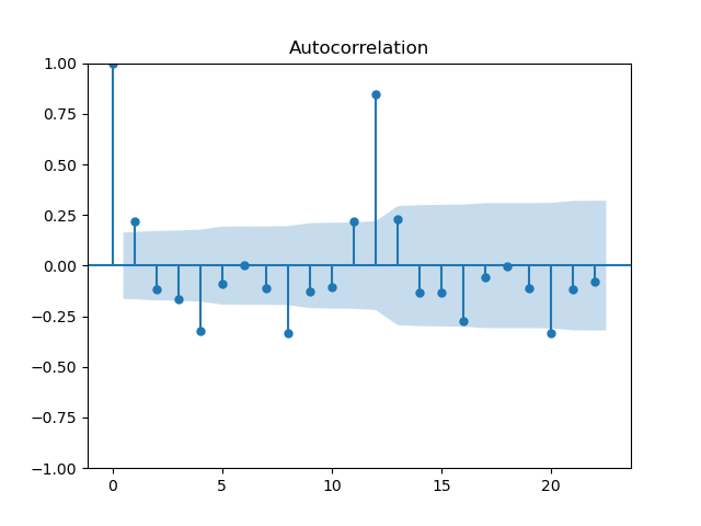
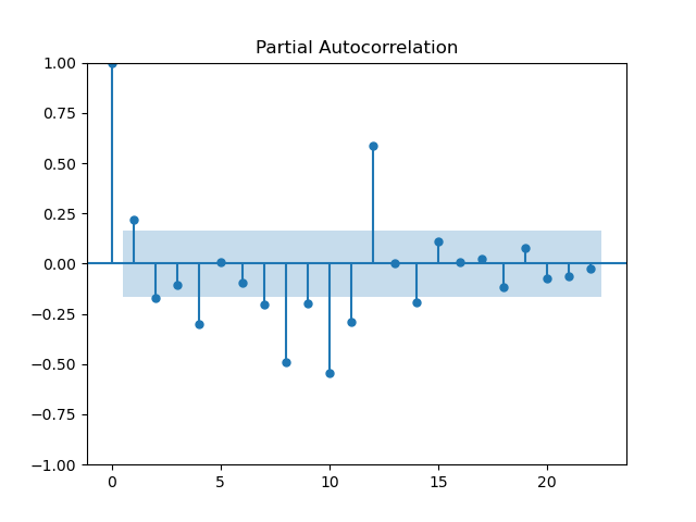
In the previous sections, I mentioned how you can find the autoregressive and moving-average orders by plotting the autocorrelation and partial autocorrelation functions. Let's show an example of how you can do it here:
Plots generated by author in Python.
The blue region signifies where the points are no longer statistically significant and from the plot we see the last lag that is statistically significant for both plot is ~12th. Therefore, we would take the order of p and q to be 12.
Now, let's fit the model using the ARIMA function and generate the forecasts:
Analysis
Plot the forecasts:
Plot generated by author in Python.
The ARIMA model has captured the data very well!
Summary and Further Thoughts
In this article we have discussed one of the most common forecasting models used in practise, ARIMA. This model combines: autoregression, differencing and moving-average models into a single univariate case. ARIMA is simple to apply in Python the statsmodels package, which does a lot of the heavy lifting for you when fitting an ARIMA model.
Full code used in this article can be found at my GitHub here:
I have a free newsletter, Dishing the Data, where I share weekly tips for becoming a better Data Scientist. There is no "fluff" or "clickbait," just pure actionable insights from a practicing Data Scientist.