Dimensionality Reduction Made Simple: PCA Theory and Scikit-Learn Implementation

Author:Murphy | View: 26706 | Time: 2025-03-22 22:57:35

In the novel Flatland, characters living in a two-dimensional world find themselves perplexed and unable to comprehend when they encounter a three-dimensional being. I use this analogy to illustrate how similar phenomena occur in Machine Learning when dealing with problems involving thousands or even millions of dimensions (i.e. features): surprising phenomena happen, which have disastrous implications on our Machine Learning models.

I'm sure you felt stunned, at least once, by the huge number of features involved in modern Machine Learning problems. Every Data Science practitioner, sooner or later, will face this challenge. This article will explore the theoretical foundations and the Python implementation of the most used Dimensionality Reduction algorithm: Principal Component Analysis (PCA).

Why do we need to reduce the number of features?

Datasets involving thousands or even millions of features are common nowadays. Adding new features to a dataset can bring in valuable information, however, they will slow the training process and make it harder to find good patterns and solutions. In Data Science this is called the Curse of Dimensionality and it often **** leads to skewed interpretation of data and inaccurate predictions.

Machine learning practitioners like us can benefit from the fact that for most ML problems, the number of features can be reduced consistently. For example, consider a picture: the pixels near the border often don't carry any valuable information. However, the techniques to safely reduce the number of features in a ML problem are not trivial and need an explanation that I will provide in this post.

The tools I will present not only simplify the computation effort and boost the prediction accuracy, but they will also serve as a tool to graphically visualize high-dimensional data. For this reason, they are essential to communicate your insights with other people.

Fortunately for us, the above-mentioned technique, named Dimensionality Reduction, exists and can easily take part in every data scientist's toolbox. Moreover, Dimensionality Reduction can be easily implemented in Python programming thanks to the Scikit-Learn (sklearn) library.

Curse of Dimensionality

The Curse of Dimensionality represents one of the biggest challenges in Data Science as it makes algorithms computationally intensive. But what is it exactly?

When the number of dimensions in a dataset grows substantially, the available data points become sparser and sparser, leading to an intricate cascade of computational challenges. As humans, we struggle to conceptualize more than 3, or sometimes 2, dimensions. This limitation leads to very unexpected behavior of data in high-dimensional spaces.

For example, consider a 2D 1×1 square. If we pick a random point inside of it, there is only a small probability for it to be located very close to a border. Numerically, there is a 0.4% probability for it to be located within a 0.001 distance from a border. Instead, in a higher-dimensional unit hypercube, as the number of edges grow, the probability for a random point to be located close to a border grows exponentially. In a 10.000-dimensional hypercube, the same probability increases to over 99.99999%. This means that in a high-dimensional space, it's very likely to be near a border.

The following experiment is even more surprising (or disturbing in my opinion). Take the usual 2-dimensional unit square. The distance of 2 randomly chosen points inside the square is, on average, equal to 0.52. Would you believe me if I tell you that doing the same experiment with a 100.000-dimensional unit hypercube results in an average distance of 129.09? I can prove that to you with the following Montecarlo simulation.

import numpy as np
test_dimensions = [2, 100000]
print('Average distance between 2 points in a unit hypercube')
for n_dim in test_dimensions:
    distances = []
    for i in range(100000):
        rand_point_1 = np.random.uniform(size=n_dim)
        rand_point_2 = np.random.uniform(size=n_dim)
        dist = np.linalg.norm(rand_point_1-rand_point_2)
        distances.append(dist)
    avg_distance = np.mean(distances)
    print('{} dimensions: {}'.format(n_dim, avg_distance))

The concept is even better represented by this visualization:

Leaving aside these funny simulations, we can extrapolate a major implication for Data Science practitioners: there is plenty of space in high-dimensions.

The consequence is that high-dimensional datasets are, with any probability, very sparse, and the training instances are far apart from each other. With such training data, the risk of overfitting your Machine Learning model is high.

While, in theory, we could add new training examples, in practice this is not enough to cope with the increase of features. In fact, in order to maintain a constant density, the required number of training points needs to grow exponentially as a function of the number of features.

Just to provide an example, to maintain a distance of 0.1 between each training point in a dataset with 100 features, we would need a number of training point greater than the number of atoms in the universe.

The only feasible approach is to reduce the number of features, and I will provide different techniques to do that while avoiding losing too much information.

Principal Component Analysis (PCA)

Principal Component Analysis (PCA) is perhaps the most popular algorithm for Dimensionality Reduction. At its functioning core, it projects the data onto a hyperplane, aiming to make the rotated features statistically uncorrelated. The rotation is typically followed by selecting a subset of these new projected features, based on their importance in describing the data.

As PCA is based on projections, it is fundamental to know what this operation is. The following section explains the Projection operation.

Projection

In practical scenarios, a vast portion of the training instances lies close to a lower-dimensional subspace of the original training set hyperspace. The reasons are:

Correlation between features: many features are heavily correlated.
Constant values: many features assume near-to-constant values.

To illustrate this concept, take the following 2D dataset:

Given the strong correlation of feature _x1 with feature _x2, we can project the dataset on a lower-dimensional plane, which, in this case, is a line. Considering the directions identified by the black arrows, called components, if we rotate the dataset such that component 1 (_p1) is horizontal, we obtain:

As the component _p2 doesn't add much information, we can project data only on component _p1.

This is, in essence, what projection does. Its effect is even clearer considering instead a 3D dataset.

We can project the original data onto a 2-dimensional plane, creating 2 new features _p1, _p2:

As there is no free meal in Machine Learning, projection is not always suited for every type of dataset. If the data, in the original feature space, belong to a plane that turns or twists, no projection operation can preserve the original information in a lower-dimensional space.

Consider for example the Swiss Roll dataset:

It consists of a 2D plane rolled over itself. In this case, we can't effectively project the data on a plane without losing a considerable portion of the original information.

To avoid this amount of information loss, we will see a different method later, which aims at "unrolling" the data.

Principal Components

As I anticipated, PCA consists of projecting the data onto a lower-dimensional hyperplane. In order to preserve as much information as possible, PCA doesn't project the data on any random hyperplane. Instead, PCA selects the hyperplane on which data projection has the maximum variance.

It is easy to understand why if we consider again a 2D example.

PCA then considers all the axes orthogonal to the one of maximum variance and selects, between them, the one with the remaining larger variance.

This process iterates as many times as the number of dimensions in the original dataset. Each identified axis is called Principal Component of the dataset.

The question now is how to mathematically compute the Principal Components. Fortunately, linear algebra provides us with the Singular Value Decomposition technique, through which we can decompose the original training set X into the matrix multiplication of 3 new matrices:

The columns of the V matrix contain the direction of all the Principal Components previously identified.

While it is easy to implement SVD with the Numpy Python library, it is even more effortless to implement PCA with the Scikit-learn (sklearn) module.

In Scikit-learn (sklearn) I first need to create a PCA() object, and later fit it on the data and transform them:

from sklearn.decomposition import PCA
from sklearn.datasets import make_swiss_roll

# Create synthetic data
X, t = make_swiss_roll(n_samples=1000, noise=0.2, random_state=42)

# Instantiate a PCA object
pca = PCA(n_components=1)

# Fit the PCA object on the data
pca.fit(X)

# Transform the data
X_transformed = pca.transform(X)

print('Original data shape: ', X.shape)
print('Transformed data shape: ', X_transformed.shape)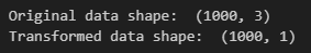

As we can see from the output, we reduced the original dataset dimension from 3 down to 1 dimension. This happened because we specified n_components=1 while instantiating the PCA() object.

Unless we are performing Dimensionality Reduction for data visualization, we might not know which is the best number of dimensions of the transformed training set.

Selecting the right number of dimensions to reduce the training set down to is a big deal in Dimensionality Reduction. If the original feature space is narrow, we might try a manual iterative approach, However, in most real-world cases, the feature space is huge and we need a more robust and automized approach.

In order to introduce said approach, I first need to define the Explained Variance Ratio (EVR). In simple terms, the EVR is defined as the percentage of the variance of the original dataset which lies along each Principal Component.

As Scikit-learn offers an intuitive explained_variance_ratio_attribute, we can apply this concept to the previous example:

from sklearn.decomposition import PCA
from sklearn.datasets import make_swiss_roll

# Create synthetic data
X, t = make_swiss_roll(n_samples=1000, noise=0.2, random_state=42)

# Instantiate a PCA object
pca = PCA(n_components=1)

# Fit the PCA object on the data
pca.fit(X)

# Calculate the EVA of each PC
eva = pca.explained_variance_ratio_

print(eva)

The variance associated with the 1st principal component is about 40%. This tells us that, by reducing the original training set dimension down to just 1 feature, we are losing about 60% of the variance.

The most straightforward approach for choosing the number of dimension of the reduced dataset is the following: use as many Principal Components as needed until the cumulative explained variance ratio reaches a given threshold.

While this approach may still appear obscure, an example will immediately clarify it. In this example, I will apply PCA on a synthetically generated dataset.

# Generate the dataset
num_instances = 10000
num_features = 784
X = np.random.rand(num_instances, num_features)

# Instantiate and train a PCA object
pca = PCA()
pca.fit(X)

# Compute the explained variance ratio
eva = pca.explained_variance_ratio_

print(np.round(eva, decimals=4)

By printing the Explained Variance Ratio of the trained PCA, we see that the first Principale Component "explains" 9.75% of the variance of the original dataset, the second Principal Component is responsible for the 7.16% of the variance, and so on. After a while, the following components' explanation of the original dataset's variance becomes negligible.

It's common practice to pick the Principal Components whose cumulative EVA values add up to 95% of the original dataset's variance:

For the synthetic dataset, we have that 153 Principal Components are able to explain 95% of the original variance. This means that, given the 784 original features, we can safely drop 631 dimensions. In other words, we can reduce by 80% the dimension of the original training set with a cost of only 5% of lost variance.

Scikit-learn (sklearn) allows us to specify the cumulative EVA threshold we want to reach, instead of the number of Principal Components to consider:

pca = PCA(n_components=.95)
pca.fit(X)
X_transformed = pca.transform(X)

print(X_transformed.shape)

In this case, we automatically get a reduced dataset made of 153 new features.

You can find all the code displayed in this post (and more) on this GitHub repository:

articles/dimensionality-reduction at main · andreoniriccardo/articles

Conclusion

In this post, we explored the theory of this powerful, and yet simple, unsupervised model. We also understood how easy it is to implement it in Python through the Scikit-Learn library.

Understanding PCA's impact on Machine Learning is essential as its applications span several industries.

I conclude this introductory guide by delineating the pros and cons of the PCA model.

The main strength of PCA is its efficiency at reducing the number of dimensions while retaining essential information, lowering computation efforts, and boosting the model's performance. It is also worth noticing that PCA decorrelates the features, meaning that the resulting Principal Components are statistically uncorrelated.

By focusing only on the most relevant features, PCA is also able to reduce the noise in the original training set.

However, as I mentioned earlier, PCA is not suited for every task. In some cases, like the Swiss Roll example, PCA is unable to fully capture the data structure. Applying PCA means transforming the original features into Principal Components, and consequently losing the interpretability of them.

Given these limitations, in my next post, I will deal with more complex Dimensionality Reduction algorithms like Kernel PCA and LLE.

As I reach the end of this guide, I need to point out that, despite having touched all the most relevant aspects of PCA, its field extends far beyond the insight provided here. For this reason, I recommend digging into the resources and references linked to this article and I encourage you to experiment with PCA on your own datasets. Your hands-on exploration will deepen your understanding, leading to valuable insights.

If you liked this story, consider following me to be notified of my upcoming projects and articles!

Here are some of my past projects: