Linear Regression In Depth (Part 1)

Author:Murphy | View: 23464 | Time: 2025-03-23 18:52:39

Linear Regression is one of the most basic and commonly used type of predictive models. It dates back to 1805, when Legendre and Gauss used linear regression to predict the movement of the planets.

The goal in regression problems is to predict the value of one variable based on the values of other variables. For example, we can use regression to predict the price of a stock based on various economic indicators or the total sales of a company based on the amount spent on advertising.

In linear regression, we assume that there is a linear relationship between the given input features and the target label, and we are trying to find the exact form of that relationship.

This article provides a comprehensive guide to both the theory and implementation of linear regression models. In the first part of the article, we will focus mainly on simple linear regression, where the data set contains only one feature (i.e., the data set consists of two-dimensional points). In the second part of the article, we will discuss multiple linear regression, where the data set may contain more than one feature.

There are many terms related to regression that data scientists often use interchangeably, but they are not always the same, such as: residuals/errors, cost/loss/error function, multiple/multivariate regression, squared loss/mean squared error/sum of squared residuals, etc.

Bearing this in mind, I have tried in this article to be as clear as possible with regard to the definitions and terminology used.

Formal Definition and Notations

Regression Problems

In regression problems, we are given a set of n labeled examples: D = {(x₁, _y_₁), (x₂, _y_₂), … , (xₙ, yₙ)}, where xᵢ represents the features of example i and yᵢ represents the label of that example.

Each xᵢ is a vector that consists of m features: xᵢ = (_xᵢ_₁, _xᵢ_₂, …, xᵢₘ)ᵗ, where ᵗ denotes the transpose. The variables xᵢⱼ are called the independent variables or the explanatory variables.

The label y is a continuous-valued variable (y ∈ R), which is called the dependent variable or the response variable.

We assume that there is a correlation between the label y and the input vector x, which is modeled by some function f(x) and an error variable ϵ:

The error variable ϵ captures all the unmodeled factors that influence the label other than the features, such as errors in the measurement or some random noise.

Our goal is to find the function f(x), since knowing this function will allow us to predict the labels for any new sample. However, since we have a limited number of training samples from which to learn f(x), we can only obtain an estimate of this function.

The function that our model estimates from the given data is called the model's hypothesis and is typically denoted by h(x).

Linear Regression

In linear regression, we assume that there is a linear relationship between the features and the target label. Therefore, the model's hypothesis takes the following form:

_w_₀, …, wₘ are called the parameters (or weights) of the model. The parameter _w_₀ is often called the intercept (or bias), since it represents the intersection point of the graph of h(x) with the _y-_axis (in two dimensions).

To simplify h(x), we add a constant feature _x_₀ that is always equal to 1. This allows us to write h(x) as the dot product between the feature vector x = (_x_₀, …, xₘ)ᵗ and the weight vector w = (_w_₀, …, wₘ)ᵗ:

Vector form of the linear regression model

Ordinary Least Squares (OLS)

Our goal in linear regression is to find the parameters _w_₀, …, wₘ that will make our model's predictions h(x) be as close as possible to the true labels y. In other words, we would like to find the model's parameters that best fit the data set.

To that end, we define a cost function (sometimes also called an error function) that measures how far our model's predictions are from the true labels.

We start by defining the residual as the difference between the label of a given data point and the value predicted by the model:

Ordinary least squares (OLS) regression finds the optimal parameter values that minimize the sum of squared residuals:

Note that a loss function calculates the error per observation and in OLS it is called the squared loss, while a cost function (typically denoted by J) calculates the error over the whole data set, and in OLS it is called the sum of squared residuals (SSR) or sum of squared errors (SSE).

Although OLS is the most common type of regression, there are other types of regression such as the least absolute deviations regression. We will motivate why the least squares function is the preferred cost function in the last section of this article.

Luckily, except for some special cases (that will be discussed later), the least squares cost function is convex. A function f(x) is convex if the line segment between any two points on the graph of the function lies above the graph. In simpler terms, the graph of the function has a cup shape ∪. This means that convex functions have only one minimum, which is also the global minimum.

Since J(w) is convex, finding its minimum points using its first-order derivatives is guaranteed to give us a unique solution, and hence the optimal one.

Simple Linear Regression

When the data set has only one feature (i.e., when it consists of two-dimensional points (x, y)), the regression problem is called simple linear regression.

Geometrically, in simple linear regression, we are trying to find a straight line that goes as close as possible through all the data points:

In this case, the model's hypothesis is simply the equation of the line:

where _w_₁ is the slope of the line and _w_₀ is its intersection with the _y-_axis. The residuals in this case are the distances between the data points and the fitted line.

In this case, the least squares cost function takes the following form:

The OLS cost function in simple linear regression

The Normal Equations

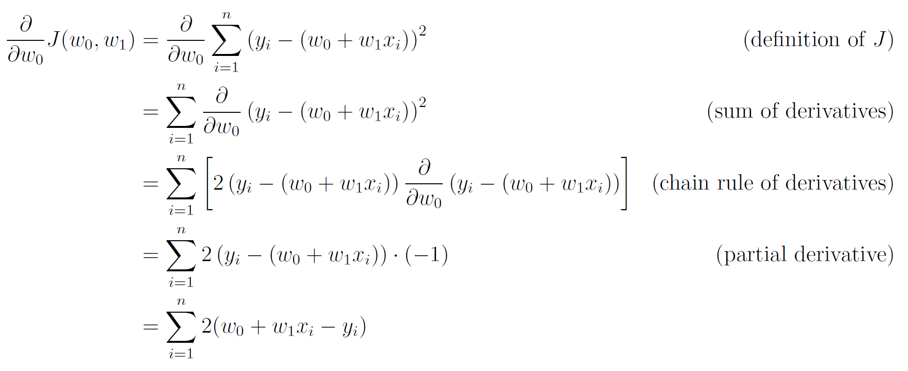
Our objective is to find the parameters _w_₀ and _w_₁ of the line that best fits the points, i.e., the line that leads to the minimum cost. To that end, we can take the partial derivatives of J(_w_₀, _w_₁) with respect to both parameters, set them to 0, and then solve the resulting linear system of equations (which are called the normal equations).

Let's start with the partial derivative of J with respect to _w_₀:

Setting this derivative to 0 yields the following:

We have found an expression for _w_₀ in terms of _w_₁ and the data points.

Next, we compute the partial derivative of J with respect to _w_₁:

Setting this derivative to 0 yields the following:

Let's substitute the expression for _w_₀ into this equation:

Therefore, the coefficients of the regression line are:

Numerical Example

Let's say that we would like to find if there is a linear correlation between the height and weight of people. We are given the following 10 examples that represent the average heights and weights of American women aged 30–39 (source: The World Almanac and Book of Facts, 1975).

To find the regression line manually, we first build the following table:

Based on the totals in the last row of the table, we can compute the coefficients of the regression line:

Therefore, the equation of the fitted line is:

Python Implementation

We will now find the regression line using Python.

First, let's write a general function to find the parameters of the regression line for any given two-dimensional data set:

def find_coefficients(x, y):
    n = len(x)
    w1 = (n * x @ y - x.sum() * y.sum()) / (n * (x**2).sum() - x.sum()**2)
    w0 = (y.sum() - w1 * x.sum()) / n
    return w0, w1

The code above is a direct translation of the normal equations into NumPy functions and operators.

Let's test our function on the same data set from above. We first define our data points:

x = np.array([1.55, 1.60, 1.63, 1.68, 1.70, 1.73, 1.75, 1.78, 1.80, 1.83])
y = np.array([55.84, 58.57, 59.93, 63.11, 64.47, 66.28, 68.10, 69.92, 72.19, 74.46])

Let's plot them:

def plot_data(x, y):
    plt.scatter(x, y)
    plt.xlabel('Height (m)')
    plt.ylabel('Weight (kg)')
    plt.grid()

plot_data(x, y)

We now find the parameters of the regression line using the function we have just written:

w0, w1 = find_coefficients(x, y)
print('w0 =', w0)
print('w1 =', w1)

w0 = -47.94681481481781
w1 = 66.41279461279636

We get the same results that we had with the manual computation, albeit with a higher precision.

Let's write another function to draw the regression line. To that end, we can simply take the minimum and maximum x values in the input range, compute their y coordinates on the regression line, and then draw the line that connects the two points:

def plot_regression_line(x, y, w0, w1):
    p_x = np.array([x.min(), x.max()])
    p_y = w0 + w1 * p_x
    plt.plot(p_x, p_y, 'r')

Lastly, let's plot the regression line together with the data points:

plot_data(x, y)
plot_regression_line(x, y, w0, w1)

We can see that the relationship between the two variables is very close to linear.

As an exercise, download the heights and weights data set from Kaggle. This data set contains the height and weight of 25,000 18-years old teenagers. Build a linear regression model for predicting the weight of a teenager from their height and plot the result.

Evaluation Metrics

There are several evaluation metrics that are used to evaluate the performance of regression models. The two most common ones are RMSE (Root Mean Squared Error) and R² score.

Note the difference between an evaluation metric and a cost function. A cost function is used to define the objective of the model's learning process and is computed on the training set. Conversely, an evaluation metric is used after the training process to evaluate the model on a holdout data set (a validation or a test set).

RMSE (Root Mean Squared Error)

RMSE is defined as the square root of the mean of the squared errors (the differences between the model's predictions and the true labels):

Note that what we called residuals during the model's training are typically called errors (or prediction errors) when they are computed over the holdout set.

RMSE is always non-negative, and a lower RMSE means the model has a better fit to the data (a perfect model has an RMSE of 0).

We can compute the RMSE directly or by using the sklearn.metrics module. This module provides numerous functions for measuring the performance of different types of models. Although it does not have an explicit function for computing RMSE, we can use the function mean_squared_error() to first find the MSE, and then take its square root to get the RMSE.

Most of the scoring functions in sklearn.metrics expect to get as parameters an array with the true labels (_ytrue) and an array with the model's predictions (_ypred). Therefore, we first need to compute our model's predictions on the given data points. This can be easily done by using the equation of the regression line:

y_pred = w0 + w1 * x

We can now call the mean_squared_error() function and find the RMSE:

from sklearn.metrics import mean_squared_error as MSE

rmse = np.sqrt(MSE(y, y_pred))
print(f'RMSE: {rmse:.4f}')

The result we get is:

RMSE: 0.5600

Advantages of RMSE:

Provides a measure for the average magnitude of the model's errors.
Since the errors are squared before they are averaged, RMSE gives a relatively higher weight to large errors.
Can be used to compare the performance of different models on the same data set.

Disadvantages of RMSE:

Cannot be used to compare the model's performance across different data sets, because it depends on the scale of the input features.
Sensitive to outliers, since the effect of each error on the RMSE is proportional to the size of the squared error.

R² Score

The _R_² score (also called the coefficient of determination) is a measure of the goodness of fit of a model. It computes the ratio between the sum of squared errors of the regression model and the sum of squared errors of a baseline model that always predicts the mean value of y, and subtracts this ratio from 1:

where ȳ is the mean of the target labels.

The best possible _R_² score is 1, which indicates that the model predictions perfectly fit the data. A constant model that always predicts the mean value of y, regardless of the input features, has an _R_² score of 0.

_R_² scores below 0 occur when the model performs worse than the worst possible least-square predictor. This typically indicates that a wrong model was chosen.

To compute the _R_² score, we can use the function r2_score from sklearn.metrics:

from sklearn.metrics import r2_score

score = r2_score(y, y_pred)
print(f'R2 score: {score:.4f}')

The result we get is:

R2 score: 0.9905

The _R_² score is very close to 1, which means we have an almost perfect model. However, note that in this example we are evaluating the model on the training set, where the model would normally have a higher score than on a holdout set.

_R_² score can also be interpreted as the proportion of the variance of the dependent variable y that is explained by the independent variables in the model (the interested reader can find why in this Wikipedia article).

Advantages of _R_² score:

Does not depend on the scale of the features.
Can be used to compare the performance of different models across different data sets.

Disadvantages of _R_² score:

Does not provide information on the magnitude of the model's errors.
_R_² score is monotonically increasing with the number of features the model has, thus it cannot be used to compare models with very different numbers of features.

OLS and Maximum Likelihood

Finally, we will show the correlation between ordinary least squares (OLS) and maximum likelihood, which is the main motivation for using OLS to solve regression problems. More specifically, we will prove that an OLS estimator is identical to the maximum likelihood estimator (MLE) under the assumption that the errors are normally distributed with zero mean.

For those unfamiliar with the concept of maximum likelihood, check out my previous article.

Recall that in linear regression we assume that the labels are generated by a linear function of the features plus some random noise:

Let's assume that the errors are independent and identically distributed (i.i.d.), and have a normal distribution with mean 0 and variance _σ_²:

In this case, the labels y are also normally distributed with a mean of wᵗx and variance _σ_² (adding a constant to a normally-distributed variable yields a variable that is also normally distributed but whose mean is shifted by that constant):

Therefore, the probability density function (PDF) of y given the inputs x and the weight vector w is:

Based on the assumption of independence of the errors (and hence the labels), we can write the likelihood of the parameters w of the model as follows:

Therefore, the log likelihood is:

We can see that the only expression in the log likelihood that depends on the parameters w is:

which is exactly the cost function of OLS! Therefore, maximizing the likelihood of the model **** is identical to minimizing the sum of squared residuals.