Early Stopping: Why Did Your Machine Learning Model Stop Training?

When training supervised machine learning models, Early Stopping is a commonly used technique to mitigate overfitting. Early stopping involves monitoring a model's performance on a validation set during training and stopping the training process once the model's performance doesn't improve on this held-out data. This technique helps save computation time and resources while ensuring that the model doesn't learn the noise and irrelevant patterns in the training data, which could reduce its ability to generalize to new, unseen data.

Early stopping is a widely recognized technique in machine learning, yet there aren't many comprehensive discussions on the specific reasons for meeting early stopping criteria in various scenarios. This article explores the intricacies of early stopping from the perspective of training data quality. By examining how data quality influences the point at which training ceases, we can gain deeper insights into its crucial role. Additionally, we will explain the fundamental differences between dealing with tabular data and unstructured data in machine learning projects, highlighting how these distinctions impact the application of early stopping techniques.

Prerequisites

Before getting started, we'll define the "random flip proportion," a technique to introduce noise into a dataset, enhancing our understanding of its impact on model training. Following this, we'll discuss early stopping in detail, including how it functions and its role in preventing overfitting. This groundwork will set the stage for a deeper investigation into the triggers and implications of early stopping.

Random Flip Proportion

Suppose we have a feature matrix, X, and a binary target, y. To artificially add noise to the data, we randomly select samples from y and replace them with a randomly selected label. We'll call the proportion of samples with randomly assigned labels the random flip proportion.

Random Flip Proportion: the proportion of samples in a classification target that have been replaced with a randomly selected label. The larger the random flip proportion, the nosier the data becomes and the harder the classification problem.

To understand this better, suppose we have a dataset with two features (x1 and x2) and a binary target. Assume that the feature space forms two unique clusters per class, and there's almost no overlap between the clusters. If we don't randomly flip any of the labels (random flip proportion = 0), the dataset might look something like this:

Because the random flip proportion is 0, we see that the features separate the class well, and we could fit a classifier that nearly perfectly predicts the target given a set of inputs (x1, x2).

Using the same dataset, if we set the random flip proportion to 0.50, then 50% of the labels will be randomly assigned to a class. The dataset might look more like this now:

We now see a much noisier dataset, and it would be nearly impossible to perfectly classify these examples. In general, as we increase the random flip proportion in a dataset, the data becomes noisier and harder to classify:

The animation illustrates that increasing the random flip proportion in the dataset introduces greater noise and complexity, making classification more challenging. At a random flip proportion of 1, where all class labels are assigned completely at random, it becomes infeasible for any classifier to perform better than random guessing.

In the next section, we'll use the random flip proportion to augment synthetic datasets and analyze the impact on early stopping. This will give us direct insight into how noise affects model training. But before we do this, let's discuss what early stopping is.

Early Stopping

Early stopping is a technique used in supervised Machine Learning to prevent overfitting during model training. Overfitting occurs when a model learns not only the underlying patterns in the training data but also the noise, leading to poor performance on new, unseen data. Early stopping aims to halt the training process at the point where performance on a validation set is optimized, with the hopes that a model generalizes well to new data.

Early stopping: a technique used in supervised machine learning to prevent overfitting during model training by halting the training process at the point where performance on a validation set is optimized.

Here's how early stopping works:

1. Training and Validation: During model training, the dataset is split into at least two parts: a training set and a validation set. The training set is used to train the model, while the validation set is used to evaluate its performance after each training iteration.
2. Monitoring Performance: As training progresses, the model's performance is continually assessed on the validation set using a predefined metric like Log Loss, F1-score, or ROC AUC.
3. Stopping Criterion: A key component of early stopping is defining a stopping criterion. For example, we might stop training if the validation loss does not improve after 20 iterations of training.
4. Model Restoration: After the stopping criterion is met, it's common practice to restore the model to the state where it performed best on the validation set.

The nature of early stopping varies depending on the model. For instance, early stopping constraints for deep learning models are often applied to the number of training epochs. That is, the neural network's performance is evaluated on the validation set after each epoch, and training is halted after performance hasn't improved over a specified number of epochs.

Tree-based ensemble models like Random Forests and Gradient Boosted Tress also benefit from early stopping. For these models, early stopping prohibits adding more trees once the performance plateaus or decreases on a validation set.

With these prerequisites converted, we can explore the fundamental causes of early stopping from a training data perspective.

Common Causes of Early Stopping

Often when a model halts training earlier than expected, we tend to blame the model architecture. While model architecture certainly influences the model's ability to learn the relationship between the feature and target, the quality of the training data plays a larger role. Let's unpack two training data characteristics that are responsible for early stopping – noisy data and informative features.

Noisy Data

The most common cause of early stopping, especially in tabular machine learning use cases, is noisy data. In this context, noisy data means the features used to train the model have little or no deterministic relationship with the target. This issue often arises when we try to predict human behaviors or financial markets due to the limited availability of data that influences these processes.

A classic example arises when we try to predict future asset prices. Any dataset used to train this kind of model will be fundamentally noisy because many of the factors that drive asset prices are unobservable. For instance, natural disasters, pandemics, human emotions, wars, and macroeconomic conditions influence asset prices, but they're difficult, if not impossible, to predict.

Early stopping occurs in the presence of noisy data because the model being trained has little or no predictive power on the validation set, and continuing to train on the noisy training set doesn't improve validation performance.

To see this, we'll create a series of synthetic datasets with varying levels of noise governed by the random flip proportion. We'll use Scikit-Learn's [make_classification()](https://scikit-learn.org/stable/modules/generated/sklearn.datasets.make_classification.html) function to create the datasets and LightGBM as the base model to train and evaluate.

We'll first define a function, evaluate_lgbm_complexity(), that creates a synthetic dataset, splits the datasets into training, validation, and test sets, trains a LightGBMClassifier with early stopping, and returns the optimal number of trees and test set ROC AUC:

Python"># early_stopping_experiment.py

from tqdm import tqdm
from sklearn.datasets import make_classification
from sklearn.model_selection import train_test_split
from lightgbm import LGBMClassifier, early_stopping
from sklearn.metrics import roc_auc_score
from sklearn.model_selection import train_test_split
from joblib import Parallel, delayed
from typing import Annotated, Any, Tuple
from pydantic import validate_call, Field

@validate_call()
def evaluate_lgbm_complexity(
    flip_prop: Annotated[float, Field(ge=0, le=1)],
    n_samples: Annotated[int, Field(gt=0)],
    n_features: Annotated[int, Field(gt=0)],
    n_informative: Annotated[int, Field(gt=0)],
    n_redundant: Annotated[int, Field(ge=0)],
    lgbm_params: dict[str, Any],
    test_prop: Annotated[float, Field(ge=0, le=1)] = 0.20,
    random_state: int = 101,
    stopping_rounds: int = 20,
) -> Tuple[int, float]:
    """
    Evaluate the performance of a LightGBM model by training it on a synthetic
    dataset generated with specified complexity parameters and computing the
    ROC AUC score.

    Parameters
    ----------
    flip_prop : float
        Proportion of the sample labels to randomly flip, with a value between
        0 and 1 inclusive.
    n_samples : int
        Number of samples to generate in the synthetic dataset.
    n_features : int
        Total number of features in the synthetic dataset.
    n_informative : int
        Number of informative features (features actually used to construct
        the target).
    n_redundant : int
        Number of redundant features (linear combinations of the informative
        features).
    lgbm_params : dict[str, Any]
        Parameters to pass to the LightGBM classifier.
    test_prop : float, optional
        Proportion of the dataset to set aside as a test set. Default is 0.20.
    random_state : int, optional
        Seed used by the random number generator. Default is 101.
    stopping_rounds : int, optional
        Number of rounds without improvement to wait before stopping training
        early. Default is 20.

    Returns
    -------
    Tuple[int, float]
        A tuple containing the number of boosting rounds used by the best
        model and the ROC AUC score of the model evaluated on the test set.
    """

    x, y = make_classification(
        n_samples=n_samples,
        n_features=n_features,
        n_informative=n_informative,
        n_redundant=n_redundant,
        flip_y=flip_prop,
        random_state=random_state,
    )

    x_train, x_test, y_train, y_test = train_test_split(
        x, y, test_size=test_prop, random_state=random_state
    )
    x_train, x_eval, y_train, y_eval = train_test_split(
        x_train, y_train, test_size=test_prop, random_state=random_state
    )

    classifier = LGBMClassifier(**lgbm_params)
    classifier.fit(
        x_train,
        y_train,
        eval_set=[(x_eval, y_eval)],
        callbacks=[
          early_stopping(stopping_rounds=stopping_rounds, verbose=False)
        ],
    )

    lgbm_params["n_estimators"] = classifier.best_iteration_

    final_classifier = LGBMClassifier(**lgbm_params)
    final_classifier.fit(
        X=np.concatenate([x_train, x_eval]),
        y=np.concatenate([y_train, y_eval])
    )

    pred_probs_classifier = final_classifier.predict_proba(x_test)[:, 1]

    roc_auc = roc_auc_score(y_test, pred_probs_classifier)

    return lgbm_params["n_estimators"], roc_auc

evaluate_lgbm_complexity() accepts the parameters needed to create the synthetic classification dataset, the parameters needed to instantiate a LGBMClassifier, the proportion of data to hold out for the test set, and the number of rounds without improvement to enact early stopping.

We then define a function, run_random_flip_experiment(), that calls evaluate_lgbm_complexity() on a range of random flip proportions and visualizes the impact on early stopping rounds and test set ROC AUC:

# early_stopping_experiment.py
...

@validate_call()
def run_random_flip_experiment(
    lgbm_params: dict[str, Any],
    n_samples: Annotated[int, Field(gt=0)],
    n_features: Annotated[int, Field(gt=0)],
    n_informative: Annotated[int, Field(gt=0)],
    n_redundant: Annotated[int, Field(ge=0)],
    test_prop: Annotated[float, Field(ge=0, le=1)] = 0.20,
    random_state: int = 101,
    stopping_rounds: int = 20,
) -> None:
    """
    Conducts an experiment to analyze the impact of randomly flipping class
    labels on the performance of a LightGBM model, particularly in terms of
    early stopping iterations and ROC AUC values across different proportions
    of flipped labels.

    Parameters
    ----------
    lgbm_params : dict[str, Any]
        Parameters to pass to the LightGBM model.
    n_samples : int
        The number of samples to generate in the dataset. Must be greater
        than 0.
    n_features : int
        The total number of features in the dataset. Must be greater than 0.
    n_informative : int
        The number of informative features. Must be greater than 0.
    n_redundant : int
        The number of redundant features. Must be non-negative.
    test_prop : float, optional
        The proportion of the dataset to be used as the test set, by default
        0.20. Must be between 0 and 1 inclusive.
    random_state : int, optional
        The random state for reproducibility, by default 101.
    stopping_rounds : int, optional
        The number of rounds for early stopping in the LightGBM model,
        by default 20.

    Returns
    -------
    None
        The function does not return any value. It produces two plots: one
        showing the relationship between the proportion of flipped labels
        and the early stopping iteration, and another showing the relationship
        between the proportion of flipped labels and the ROC AUC score.

    Notes
    -----
    This experiment is intended to help understand how model robustness
    varies as a function of label noise introduced by flipping the class
    labels at random. The `Parallel` execution and the `tqdm` progress bar
    are used for efficient computation and real-time progress updates
    respectively.
    """

    flip_props = np.arange(0.02, 1.02, 0.02)

    joblib_args = [
        (
            flip_prop,
            n_samples,
            n_features,
            n_informative,
            n_redundant,
            lgbm_params,
            test_prop,
            random_state,
            stopping_rounds,
        )
        for flip_prop in flip_props
    ]

    results = Parallel(n_jobs=-1)(
        delayed(evaluate_lgbm_complexity)(*joblib_arg)
        for joblib_arg in tqdm(joblib_args)
    )
    early_stopping_iterations, roc_auc = zip(*results)

    fig, ax = plt.subplots(figsize=(10, 6))
    ax.scatter(flip_props, early_stopping_iterations)
    ax.set_xlabel("Random Flip Proportion")
    ax.set_ylabel("Early Stopping Iteration")
    ax.set_title("Stopping Iteration vs Random Class Flip Proportion")
    plt.show()

    fig, ax = plt.subplots(figsize=(10, 6))
    ax.scatter(flip_props, roc_auc)
    ax.set_xlabel("Random Flip Proportion")
    ax.set_ylabel("ROC AUC")
    ax.set_title("ROC AUC vs Random Class Flip Proportion")
    plt.show()

Crucially, run_random_flip_experiment() allows us to fix the parameters of the LightGBM classifier, along with the characteristics of the training data, and isolate the effect of the random flip proportion on early stopping __ and ROC AUC.

Lastly, we call run_random_flip_experiment() with the following parameters and visualize the results:

# early_stopping_experiment.py

...

if __name__ == "__main__":

    n_samples = 100_000
    n_features = 40
    n_informative = n_features - 1
    n_redundant = 0
    test_prop = 0.20
    random_state = 101
    stopping_rounds = 20

    lgbm_params = {
        "n_estimators": 20_000,
        "learning_rate": 0.01,
        "max_depth": 4,
        "verbose": -1,
    }

    run_random_flip_experiment(
        lgbm_params,
        n_samples,
        n_features,
        n_informative,
        n_redundant,
        test_prop,
        random_state,
        stopping_rounds,
    )

This synthetic dataset has 100,000 samples and 40 features. We hold out 20,000 samples for testing, 6,000 samples for validation, and training terminates after 20 iterations without improvement on the validation set.

The LightGBM classifier will have 20,000 trees (unless the early stopping occurs), a learning rate of 0.01, and a max depth of 4. With these dataset and model parameters, run_random_flip_experiment() will iteratively add noise to the data and assess the impact on early stopping and ROC AUC.

Here's what the results look like:

As the random flip proportion increases, there's a clear decrease in the early stopping iteration. When the random flip proportion is 0, meaning the relationship between the features and target is nearly deterministic, the LightGBM classifier trains for 16,000 of the 20,000 allowed iterations before hitting early stopping on the validation set. As more noise is added, the early stopping iteration drops off steeply.

When the random flip proportion is 1, the relationship between the features and target is completely random, and the model hits the early stopping criteria after the first 20 iterations. Training on a random data set doesn't teach the model anything useful that would help it generalize to out-of-sample data. This is why we see early stopping take effect almost immediately.

We can also analyze what happens to classification performance on the test set as we increase the random flip proportion:

The higher the random flip proportion, the worse the model performs on the test set. When the data is noiseless (random flip proportion = 0), the model trains for 16,000 iterations and achieves near-perfect performance on the test set. As the random flip proportion increases, the model's test set performance decreases until it eventually becomes random guessing (ROC AUC = 0.50).

This experiment indicates a lot about the impact of noise on early stopping. The main takeaway is that the noisier the data, the quicker a model will hit early stopping criteria. This suggests that, when our models stop training earlier than expected, we should ask "Are the features I'm using sufficient to predict the target?". Of course, the answer to this question can be subjective since the predictive power of the features lies on a spectrum from useless (random flip proportion = 1) to completely deterministic (random flip proportion = 0). However, early stopping might suggest that our features have less predictive power than we expected.

Up next, we'll look at another common property of the training data that can cause early stopping – informative features.

Informative Features

Another possible cause of early stopping is the number of informative features in the training data. Informative features are any features in the data used to generate the target. For example, suppose we have three available features, x1, x2, and x3, and the target is generated according to the equation *f(x1, x2) = x1x2 + ε. In this case, x1 and x2 are informative features because they're explicitly used to generate the target, while x3 is uninformative because it doesn't affect the target. We also assume that x3 is independent of x1 and x2, so including x3** in a model will have no predictive benefit.

To assess the effect of informative features on early stopping, we'll run a similar experiment as we did before. Our synthetic dataset will have 100,000 samples and 40 total features. We'll set the random flip proportion to 0.20 to add a slight amount of noise to the data. We'll hold out 20,000 samples for testing, 6,000 samples for validation, and training will terminate after 20 iterations without improvement on the validation set.

The key difference in this experiment is that, instead of varying the random flip proportion, we'll vary the number of informative features. The first model will have 1 informative feature out of 40, the second model 2 informative features, and so on. Here's what the results look like:

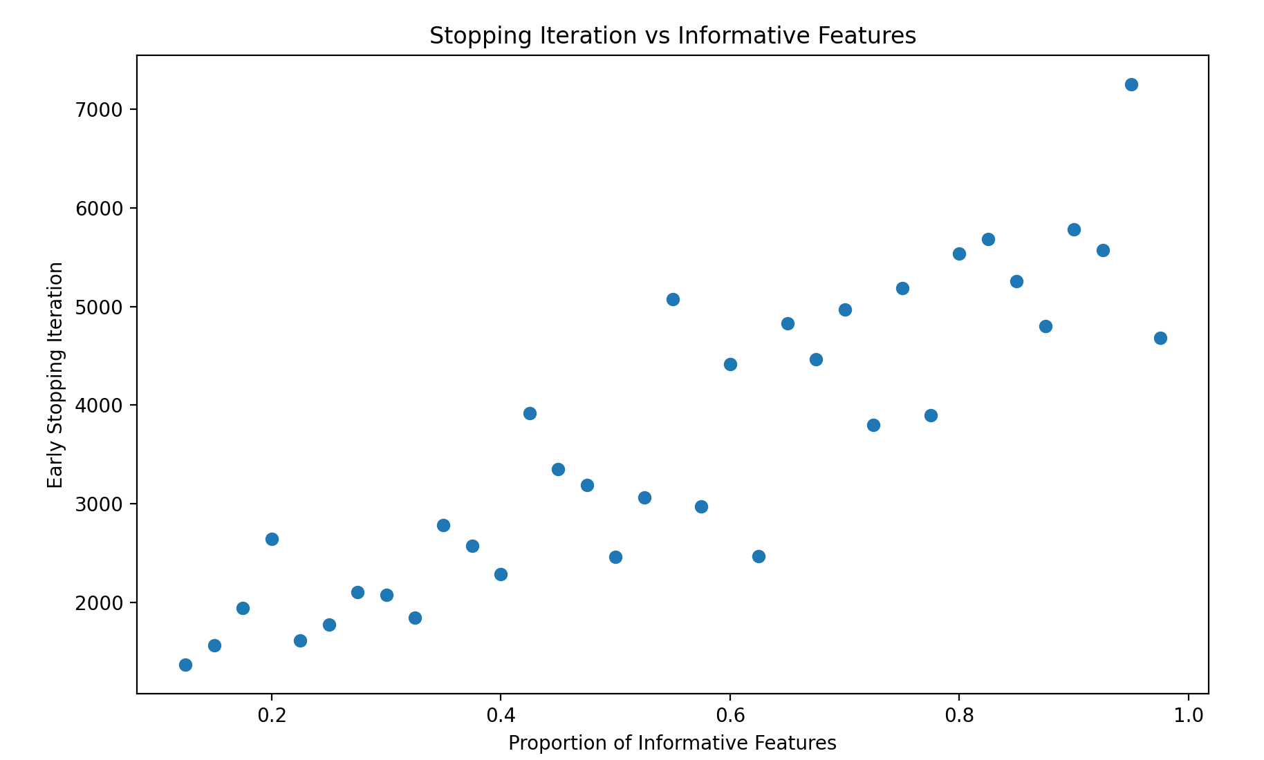
While the relationship between informative features and early stopping isn't quite as strong as in the random flip experiment, we see a clear trend. As the proportion of informative features increases, the dataset becomes more complex, and the model requires more iterations to learn the relationship between the features and the target. When there is only one informative feature, the model learns the relationship between the features and target in a small number of iterations. As more features are used to generate the target, the model tends to use more iterations to learn the relationship.

Next, let's analyze how the proportion of informative features relates to ROC AUC:

Interestingly, the proportion of informative features doesn't have a clear relationship with ROC AUC. This makes sense because the random flip proportion is fixed and is essentially the only dataset characteristic that impacts a classifier's achievable performance. For a fixed amount of noise, increasing the proportion of informative features doesn't necessarily result in better classification performance. However, as the proportion of informative features increases, larger models are required to optimally fit the training data.

Why Most Models are Small and LLMs are Large

The two experiments we ran were conducted on fixed tabular datasets using LightGBM classifiers, and we can't necessarily make definitive statements about the nature of early stopping in machine learning from these. However, these experiments are consistent with the following hypothesis:

1. In many tabular machine learning use cases like loan default prediction, asset pricing, anomaly detection, and fraud detection, the datasets are riddled with noise and often have a low number of informative features relative to the number of available features. For models trained on these datasets, early stopping criteria are often met quickly because there is no benefit from a large number of training iterations.
2. In natural language processing, and more specifically generative language modeling, the training data (i.e. language) is extraordinarily high dimensional and contains relatively little noise. These characteristics explain why increasing the size and complexity of language models results in increasingly better performance. Said differently, because language data is so complex and rich in information, early stopping criteria are seldom met when training language models.

The main idea behind the first hypothesis is that tabular datasets tend to be noisy and incomplete, and often only a few features significantly enhance a model's ability to predict the target. In these settings, models quickly reach a point during training where additional iterations do not improve performance, activating early stopping criteria. This phenomenon prevents overfitting and reduces computational expense but also limits the size and complexity of the models that are typically used.

With language models, the scenario is completely different. The data used to train language models encapsulates a broad spectrum of human knowledge and language nuances, which are both high-dimensional and rich in contextual information. This abundance and diversity of data mean that language models benefit from additional training iterations and larger model architectures. As these models train longer, they tend to generate more accurate, coherent, and contextually appropriate outputs.

Thus, the training process for language models often involves much longer periods before reaching early stopping criteria, if they are used at all, allowing these models to grow significantly larger without the drawbacks of overfitting that are commonly seen in tabular data scenarios. Of course, there are diminishing returns, but this stark difference in data characteristics and training dynamics is what underpins the divergence in model sizes between tabular machine learning applications and language modeling.

Final Thoughts

In exploring the role of early stopping in machine learning training processes, this tutorial intended to shed light on ways that data quality impacts model training. By examining both the random flip proportion and the number of informative features, we've gained insights into the dynamics that trigger early stopping. These experiments highlight that not all data challenges are equal – some, like excessive noise, call for early intervention, while others, such as insufficient informative features, may allow for more extensive exploration before necessitating a halt.

While smaller models in noisy, feature-sparse environments benefit quickly from early stopping, the richer, more complex datasets typical of LLMs justify longer training durations and larger model architectures, allowing them to extract deeper patterns and nuances without the same risk of overfitting.

As machine learning practitioners, the key takeaway is to tailor early stopping strategies to the specific characteristics of our data and the operational demands of our models. This ensures optimal performance and efficiency, safeguarding the delicate balance between underfitting and overfitting. Understanding and applying these principles will enhance our ability to deploy robust, generalizable models across a variety of domains and challenges.

Tags: Data Science Early Stopping Hands On Tutorials Machine Learning Python

Comment