How to Detect Hallucinations in LLMs

Who is Evelyn Hartwell?

Evelyn Hartwell is an American author, speaker, and life coach…

Evelyn Hartwell is a Canadian ballerina and the founding Artistic Director…

Evelyn Hartwell is an American actress known for her roles in the…

No, Evelyn Hartwell is not a con artist with multiple false identities, living a deceptive triple life with various professions. In fact, she doesn't exist at all, but the model, instead of telling me that it doesn't know, starts making facts up. We are dealing with an Llm Hallucination.

Long, detailed outputs can seem really convincing, even if fictional. Does it mean that we cannot trust chatbots and have to manually fact-check the outputs every time? Fortunately, there could be ways to make chatbots less likely to say fabricated things with the right safeguards.

For the outputs above, I set a higher temperature of 0.7. I am allowing the LLM to change the structure of its sentences in order not to have identical text for each generation. The differences between outputs should be just semantic, not factual.

This simple idea allowed for introducing a new sample-based hallucination detection mechanism. If the LLM's outputs to the same prompt contradict each other, they will likely be hallucinations. If they are entailing each other, it implies the information is factual. [2]

For this type of evaluation, we only require the text outputs of the LLMs. This is known as black-box evaluation. Also, because we don't need any external knowledge, is called zero-resource. [5]

Sentence embeddings cosine distance

Let's start with a very basic way of measuring similarity. We will compute the pairwise cosine similarity between corresponding pairs of embedded sentences. We normalize them because we need to focus only on the vector's direction, not magnitude. The function below takes as input the originally generated sentence called output and a list of 3 sample outputs called _sampledpassages. All the completions are found in the image at the beginning of the article.

For generating the embeddings, I am using the all-MiniLM-L6-v2 lightweight model. Embedding a sentence turns it into its vectorial representation.

output = "Evelyn Hartwell is a Canadian dancer, actor, and choreographer." 
output_embeddings= model.encode(output)

array([ 6.09108340e-03, -8.73148292e-02, -5.30637987e-02, -4.41815751e-03,
 1.45469820e-02, 4.20340300e-02, 1.99541822e-02, -7.29453489e-02,
...
 -4.08893749e-02, -5.41420840e-02, 2.05906332e-02, 9.94611382e-02,
 -2.24501686e-03, 2.29083393e-02, 7.80007839e-02, -9.53456461e-02],
 dtype=float32)

We generate embeddings for every output of the LLM; then, we compute the pairwise cos similarity using the _pairwise_cossim function from sentence_transformers. We'll compare the original response to each new sample response and then do the average.

from sentence_transformers.util import pairwise_cos_sim
from sentence_transformers import SentenceTransformer

def get_cos_sim(output,sampled_passages):
    model = SentenceTransformer('all-MiniLM-L6-v2')
    sentence_embeddings = model.encode(output).reshape(1, -1)
    sample1_embeddings = model.encode(sampled_passages[0]).reshape(1, -1)
    sample2_embeddings = model.encode(sampled_passages[1]).reshape(1, -1)
    sample3_embeddings = model.encode(sampled_passages[2]).reshape(1, -1)
    cos_sim_with_sample1 = pairwise_cos_sim(
    sentence_embeddings, sample1_embeddings
    )
    cos_sim_with_sample2  = pairwise_cos_sim(
    sentence_embeddings, sample2_embeddings
    )
    cos_sim_with_sample3  = pairwise_cos_sim(
    sentence_embeddings, sample3_embeddings
    )
    cos_sim_mean = (cos_sim_with_sample1 + cos_sim_with_sample2 + cos_sim_with_sample3) / 3
    cos_sim_mean = cos_sim_mean.item()
    return round(cos_sim_mean,2)

This is the intuition behind how the function works with a very simple pair of vectors in a 2D cartesian space. A and B are the original vectors, and  and B̂ are the normalized ones.

From the image above, we can see that the angle between the vectors is approximately 30⁰, so they are close to each other. The cosine is approximately 0.87. The closer the cosine is to 1, the closer the vectors are to each other.

cos_sim_score = get_cos_sim(output, [sample1,sample2,sample3])

The _cos_simscore for our embedded outputs has an average value of 0.52.

To understand how to interpret this number, let's compare it to the cosine similarity score for some valid outputs where we ask for information about an existing person.

The pairwise cosine similarity score, in this case, is 0.93. Looks promising, especially as it's a very fast method of assessing the similarity between outputs.

SelfCheckGPT- BERTScore

The BERTScore builds on the pairwise cosine similarity idea we implemented previously.

The default tokenizer for computing the contextual embeddings is RobertaTokenizer. Contextual embeddings differ from static embeddings because they take into account the context around the word. For example, the word "bat" would correspond to different token values depending on whether the context refers to a "flying mammal" or a "baseball bat".

def get_bertscore(output, sampled_passages):
    # spacy sentence tokenization
    sentences = [sent.text.strip() for sent in NLP(output).sents] 
    selfcheck_bertscore = SelfCheckBERTScore(rescale_with_baseline=True)
    sent_scores_bertscore = selfcheck_bertscore.predict(
        sentences = sentences, # list of sentences
        sampled_passages = sampled_passages, # list of sampled passages
    )
    df = pd.DataFrame({
    'Sentence Number': range(1, len(sent_scores_bertscore) + 1),
    'Hallucination Score': sent_scores_bertscore
    })
    return df

Let's take an inside look at the _selfcheckbertscore.predict function. Instead of passing the full original output as an argument, we split it into individual sentences.

['Evelyn Hartwell is an American author, speaker, and life coach.',
 'She is best known for her book, The Miracle of You: How to Live an Extraordinary Life, which was published in 2007.',
 'She is a motivational speaker and has been featured on TV, radio, and in many magazines.',
 'She has authored several books, including How to Make an Impact and The Power of Choice.']

This step is important because the s_elfcheckbertscore.predict function computes the BERTScore for each sentence into the original response matched to each sentence from the samples. First, it creates an array with the number of rows equal to the number of sentences in the original output and the number of columns equal to the number of samples.

array([[0., 0., 0.],
       [0., 0., 0.],
       [0., 0., 0.],
       [0., 0., 0.]])

The model used for computing the BERTScore between the candidate and reference sentences is RoBERTa large with 17 layers. Our original output has 4 sentences, which I will call r1,r2,r3, and r4. The first sample has two sentences: c1 and c2. We compute the F1 BERTScore for each sentence from the original output matched to each sentence from the first sample. Then we do base rescaling with respect to the baseline tensor b = tensor([0.8315, 0.8315, 0.8312]). The baseline b was computed using 1 million randomly paired sentences from the Common Crawl monolingual datasets. They computed the BERTScore for each pair and averaged it. This represents a lower bound since random pairs have little semantic overlap. [1]

We keep the BERTScore of each sentence from the original response with the most similar sentence from each drawn sample. The logic is that if a piece of information appears across multiple samples generated from the same prompt, there is a good chance that the information is factual. If a statement only appears in one sample and not in any other samples from the same prompt, it is more likely to be a fabrication.

Let's add the maximum similarities in the array for the first sample:

bertscore_array
array([[0.43343216, 0.        , 0.        ],
       [0.12838356, 0.        , 0.        ],
       [0.2571277 , 0.        , 0.        ],
       [0.21805632, 0.        , 0.        ]])

Now we repeat the process for the other two samples:

array([[0.43343216, 0.34562832, 0.65371764],
       [0.12838356, 0.28202596, 0.2576825 ],
       [0.2571277 , 0.48610589, 0.2253703 ],
       [0.21805632, 0.34698656, 0.28309497]])

Then we compute the mean for each row, giving us the similarity score between each sentence from the original response and each subsequent sample.

array([0.47759271, 0.22269734, 0.32286796, 0.28271262])

The hallucination score for each sentence is obtained by subtracting from 1 each of the values above.

Comparing the results with the answers for Nicolas Cage.

Seems reasonable; the hallucination score for the valid outputs is low, and the one for the made-up outputs is high. Unfortunately, the process of computing the BERTScore is very time-consuming, which makes it a bad candidate for real-time hallucination detection.

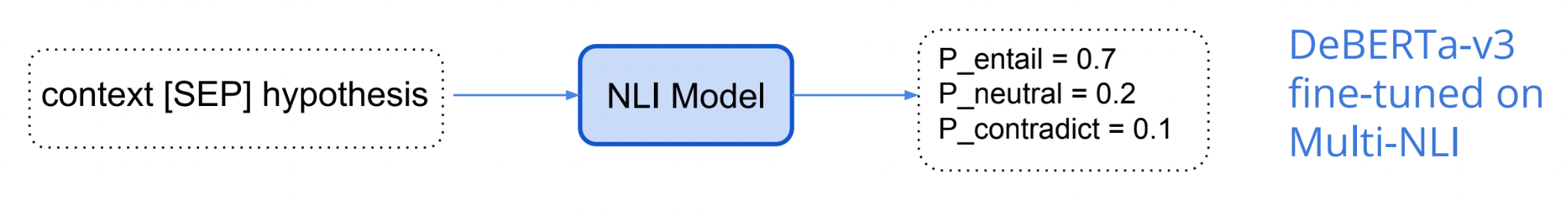
SelfCheckGPT-NLI

Natural language inference (NLI) involves determining whether a hypothesis logically follows from or contradicts a given premise. The relationship is classified as entailment, contradiction, or neutral. For SelfCheck-NLI, we utilize the DeBERTa-v3-large model that has been fine-tuned on the MNLI dataset to perform NLI.

Below are some examples of premise-hypothesis pairs and their labels.

def get_self_check_nli(output, sampled_passages):
    # spacy sentence tokenization
    sentences = [sent.text.strip() for sent in nlp(output).sents] 
    selfcheck_nli = SelfCheckNLI(device=mps_device) # set device to 'cuda' if GPU is available
    sent_scores_nli = selfcheck_nli.predict(
        sentences = sentences, # list of sentences
        sampled_passages = sampled_passages, # list of sampled passages
    )
    df = pd.DataFrame({
    'Sentence Number': range(1, len(sent_scores_nli) + 1),
    'Probability of Contradiction': sent_scores_nli
    })
    return df

In the _selfchecknli.predict function, each sentence from the original response is paired with each of the three samples.

logits = model(**inputs).logits # neutral is already removed
probs = torch.softmax(logits, dim=-1)
prob_ = probs[0][1].item() # prob(contradiction)

Now we repeat the process for each of the four sentences.

We can see that the model is outputting an extremely high probability of contradiction. Now we compare with the factual outputs.

The model is doing a great job! Unfortunately, the NLI check is a bit too long.

SelfCheckGPT-Prompt

Newer methods have started using LLMs themselves to evaluate generated text. Instead of using a formula to calculate a score, we will send the output along with the three samples to gpt-3.5-turbo. The model will decide how consistent the original output is with respect to the other three samples generated. [3]

def llm_evaluate(sentences,sampled_passages):
    prompt = f"""You will be provided with a text passage 
                and your task is to rate the consistency of that text to 
                that of the provided context. Your answer must be only 
                a number between 0.0 and 1.0 rounded to the nearest two 
                decimal places where 0.0 represents no consistency and 
                1.0 represents perfect consistency and similarity. nn 
                Text passage: {sentences}. nn 
                Context: {sampled_passages[0]} nn 
                {sampled_passages[1]} nn 
                {sampled_passages[2]}."""

    completion = client.chat.completions.create(
    model="gpt-3.5-turbo",
    messages=[
        {"role": "system", "content": ""},
        {"role": "user", "content": prompt}
    ]
    )

    return completion.choices[0].message.content

The self-similarity score returned for Evelyn Hartwell is 0. Meanwhile, the score for the outputs related to Nicolas Cage is 0.95. The time needed for getting the score is also pretty low.

This seems to be the best solution for our case, as we were also expecting from the comparative analysis of the source paper [2]. SelfCheckGPTPrompt significantly outperformed all other methods, with NLI being the second-best performing method.

The evaluation dataset was created by generating synthetic Wikipedia articles using the WikiBio dataset and GPT-3. To avoid obscure concepts, 238 article topics were randomly sampled from the top 20% of the longest articles. GPT-3 was prompted to generate the first paragraphs in a Wikipedia style for each concept.

Next, these generated passages were manually annotated for factuality at the sentence level. Each sentence was labeled as major inaccurate, minor inaccurate, or accurate based on predefined guidelines. In total, 1908 sentences were annotated, with around 40% major inaccurate, 33% minor inaccurate, and 27% accurate.

To assess annotator agreement, 201 sentences had dual annotations. If the annotators agreed, that label was used; otherwise, the worst-case label was chosen. Inter-annotator agreement measured by Cohen's kappa was 0.595 when selecting between accurate, minor inaccurate, and major inaccurate and 0.748 when minor/major inaccuracies were combined into one label.

The evaluation metric, AUC-PR, refers to the area under the precision-recall curve, which is a metric used to evaluate classification models.

Real-time hallucination detection

As a final application, let's build a Streamlit app for real-time hallucination detection. As mentioned before, the best metric is the LLM self-similarity score. We will use a threshold of 0.5 to decide whether to display the generated output or a disclaimer.

import streamlit as st
import utils
import pandas as pd

# Streamlit app layout
st.title('Anti-Hallucination Chatbot')

# Text input
user_input = st.text_input("Enter your text:")

if user_input:

    prompt = user_input

    output, sampled_passages = utils.get_output_and_samples(prompt)

    # LLM score
    self_similarity_score = utils.llm_evaluate(output,sampled_passages)

    # Display the output
    st.write("**LLM output:**")
    if float(self_similarity_score) > 0.5:
        st.write(output)
    else:
        st.write("I'm sorry, but I don't have the specific information required to answer your question accurately. ")

Now, we can visualize the final result.

Conclusion

The results are very promising! Hallucination detection in chatbots has been a long-discussed quality problem.

What makes the techniques outlined here so exciting is the novel approach of using an LLM to evaluate the outputs of other LLMs. Specifically done by generating multiple responses to the same prompt and comparing their consistency.

There is still more work to be done, but rather than relying on human evaluation or hand-crafted rules, it seems to be a good direction to let the models themselves catch the inconsistencies.

. . .

If you enjoyed this article, join Text Generation – our newsletter has two weekly posts with the latest insights on Generative AI and Large Language Models.

You can find the full code for this project on GitHub.

You can also find me on LinkedIn.

. . .

References:

1. BERTSCORE: EVALUATING TEXT GENERATION WITH BERT
2. SELFCHECKGPT: Zero-Resource Black-Box Hallucination Detection for Generative Large Language Models
3. https://learn.deeplearning.ai/quality-safety-llm-applications

4. A Broad-Coverage Challenge Corpus for Sentence Understanding through Inference

5. https://drive.google.com/file/d/13LUBPUm4y1nlKigZxXHn7Cl2lw5KuGbc/view
6. https://drive.google.com/file/d/1EzQ3MdmrF0gM-83UV2OQ6_QR1RuvhJ9h/view

Tags: Artificial Intelligence ChatGPT Generative Ai Tools Llm NLP

Comment