How to Handle Time Series Missing Data
Introduction
Problems in data collection can cause missing data. This issue can arise due to various reasons, such as sensor maintenance or transmission failure.
Missing data is usually solved by data imputation strategies, such as replacing the missing value with a central statistic. For time series, the imputation process is more challenging because the observations are ordered. Besides that, it may be useful to choose a strategy that considers the mechanism that causes missing data.
In this article, you'll learn the main patterns of time series missing data, and how to deal with them.
What causes missing data and why it matters
The patterns of missing data, such as their frequency, depend on the mechanism that causes the missingness.
Generally, the cause of missing data falls into one of the following categories:
- Missing Completely at Random: When there's no systematic process that causes an observation to miss. So, the missingness is unrelated to both 1) the value of the observation and 2) the past or future values and whether these are also missing. Many examples fall into this category, such as random sensor malfunctions or data corruption during transmission.
- Missing at Random: When the missing value is related to other values in the series, though not related to the value itself (i.e. if it's high or low). An example is when equipment is shut down for maintenance, so the sensor stops transmitting data for some period that spans several observations.
- Not Missing at Random: The missing observation depends on its value and it can also depend on other variables or observations. For example, a temperature sensor fails during periods of extreme heat conditions.
Understanding the mechanism that causes missing data can help you choose an appropriate imputation strategy. This can improve the robustness of models and analyses.
How to deal with missing data in time series
Before jumping into different methods to deal with missing values, let's prepare a time series to run some examples:
import numpy as np
from datasetsforecast.m3 import M3

# loading a time series from M3
dataset, *_ = M3.load('./data', 'Quarterly')

series = dataset.query(f'unique_id=="Q1"')

# simulating some missing values
## in this case, completely at random
series_with_nan = series.copy()

n = len(series)

na_size = int(0.3 * n)

idx = np.random.choice(a=range(n), size=na_size, replace=False)

series_with_nan[idx] = np.nan
In the preceding code, we load a time series using the datasetsforecast library. Then, we remove some of the observations to simulate missing data. In this case, we remove observations completely at random.

Let's learn about a few methods to deal with missing values.
Forward and backward propagation
Forward filling is a simple imputation strategy that relies on the sequential nature of time series. It works by filling in missing values using the most recent known observation.
# forward propagation
series_with_nan.ffill()
Backward filling is a similar approach, but uses the next non-missing observation to fill in missing values.
# backward propagation
series_with_nan.bfill()
The forward version is preferable to avoid data leakage since it doesn't introduce future information.
If your series contains a seasonal part, you can also try to use known values from the same season. Alternatively, decompose the series before filling in missing values.
Forward or backward filling can introduce bias if the missingness is related to the unobserved value. That is, when the missing data mechanism is of the type Not Missing at Random.
Usually, imputation works best if you can use data from both sides, past and future. Below are some examples to do this. Yet, you should be cautious not to introduce biases or data leakage by using future information.
Imputation using the average
A simple imputation technique, for time series and other types of data, is the mean.
series_with_nan.fillna(series_with_nan.mean())Mean imputation is usually avoided when working with time series because the temporal aspect is disregarded. Besides, there's an implicit assumption of stationarity that may not be met.
You can mitigate the limitations of this method by using a moving average. Here's an example:
series_with_nan.fillna(series_with_nan.rolling(window=5, min_periods=1).mean()).plot()A moving average is better at adapting to changes by considering a few nearby data points to compute the mean. Yet, it can still lead to biased results if the data is not missing at random.
Interpolation
You can use interpolation to impute missing data. Interpolation methods aim to estimate the value of observations that fall between known values.
A linear interpolation method works by assuming a linear relationship between the observed points and drawing a straight line accordingly. Here's how to use it for time series imputation:
series_with_nan.interpolate(method='linear')There are other interpolation methods besides the linear one, such as polynomial curves or splines.
series_with_nan.interpolate(method='polynomial', order=2)
series_with_nan.interpolate(method='spline')
You can explore the documentation of the interpolate method from pandas for a list of interpolation approaches.
Interpolation is an effective approach to impute missing values in time series. It works best if the time series is reasonably smooth. In case there are sudden changes or outliers, a simpler approach such as forward filling might be a better option.
The following figure shows the application of some of the above methods to the example time series.

Besides imputation, you may consider dropping missing values.
Dropping missing data
Removing incomplete observations is a simple solution to handle missing data.
Dropping missing values can be a reasonable option if the sample size is large enough so that there's no significant loss of information. You need to make sure that removing missing data does not introduce some sort of selection bias. Again, in cases where data is not missing at random, for instance.
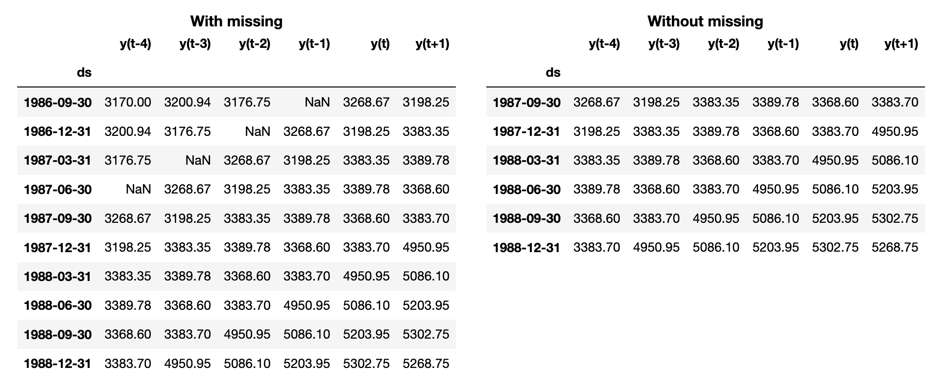
Let's see an example where we drop missing values as part of the preprocessing steps before building a Forecasting model. First, we convert the time series into a tabular format using a sliding window:
# transforming time series using a sliding window
df = series_as_supervised(series_with_nan, n_lags=5, horizon=1)

# dropping instances with missing values
df.dropna()
In the preceding code, we drop any timestep that contains at least one missing value using dropna.
Here's a sample of this dataset, with and without the missing data:
You can read a previous article to learn more about transforming a time series for supervised learning.
Takeaways
Missing data plagues all types of datasets, including time series. This issue can be caused by different factors, which may or may not be random.
You should take into account the mechanism that causes missing data when selecting a strategy to deal with missing values. In this article, we outlined a few approaches for Imputation, such as:
- forward or backward filling
- average imputation
- interpolation
We also explored when dropping missing values can be a reasonable solution, and how to do that.
Thank you for reading, and see you in the next story.
Code
References
- Moritz, Steffen, and Thomas Bartz-Beielstein. "imputeTS: time series missing value imputation in R." R J. 9.1 (2017): 207.
- Jamshidian, Mortaza, Siavash Jala Jalal, and Camden Jansen. "MissMech: An R package for testing homoscedasticity, multivariate normality, and missing completely at random (MCAR)." Journal of Statistical software 56.6 (2014): 1–31.
