How To Solve Optimization Problems Using Linear Programming

Background
Linear programming (LP) is an Optimization technique that is used to find the best solution, from a specified objective function, subject to some constraints. It is applied in sundry industries ranging from finance to e-commerce, so it's well worth knowing if you are a Data Scientist. The key feature of LP is the linear __ part, which means that the constraints and objective function are all formulated as a linear relationship. In this post, we will run through an example LP problem and how it can be solved using the simplex algorithm and the graphical method.
Graphical Method
Basic Problem
We will start with the graphical method as thats the simplest to understand and gives us real intuition behind LP.
Let's say we run a small business selling smoothies for £3 and coffees for £2, these are our two decision variables. Due to our ingredient constraints, we can only produce 75 smoothies and 100 coffees daily. Furthermore, we only have 140 cups available each day to serve our smoothies and coffees. Now, let's formulate this as an LP problem!
Formulation
If we let x be smoothies and y be coffee, then we want to maximise the following objective function, c, as a function of the decision variables:

Subject to the following constraints:

The decision variables need to be non-negative.
Now it is time to plot these constraints!
Plotting
As this is a two-dimensional problem, we can plot the constraints on a cartesian graph as straight lines (the linear part!):
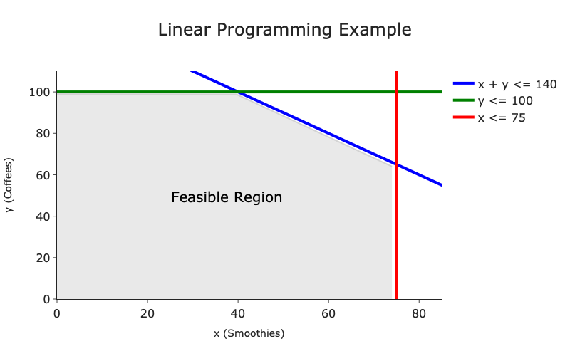
The grey area is known as the feasible region, where any solution is valid as it satisfies the constraint.
From viewing the plot, the optimal solution appears to be in one of the corners where the constraints' lines cross. This is actually called the fundamental theorem of linear programming. This theorem states that the optimal (maxima) of a linear function is in the corners over a convex polygon region (the feasibility region).
The optimal solution here is the (75, 65) corner with a value of £355. This can simply be derived from testing each corner of the feasible region.
Limitation
The above example is very simple to understand, however, what happens if we have another two products that our business sells? Well, it then becomes a four-dimensional problem. However, we humans can't visualise that on paper. So what do we do? Well as every Data Scientist knows, we use an algorithm!
Simplex Algorithm
Intuition
The simplex algorithm was invented to solve LP problems by George Dantzig during the second world war. The general flow of the algorithm is to go to every vertex of the convex polygon and evaluate the objective function. Once we reach the optimal solution (we will show how we know it's optimal), then we terminate the algorithm.
In my opinion, the best way to learn the simplex algorithm is to apply it to a problem and explain what each step is doing. So, without further ado, let's get into it!
The mathematical proof behind the algorithm is quite dense, so I haven't gone into all the gritty details in this post. However, the interested reader can find it linked here.
Walk Through
Step 1:
Transform the inequalities into a system of linear equations through the use of slack variables:

Here _s_1, s_2, and s_3_ are the slack variables, which literally pick up the slack enabling the inequalities to turn into equations. The slack variables are referred to as basic variables and the decision variables, x and y, are non-basic variables.
Step 2:
Construct the equations into a tableau, where each equation is given its own row and the objective function is the bottom row:

This is known as the initial basic solution and corresponds to the (0,0) vertex in the plot we showed earlier.
Step 3:
Next, we need to identify the pivot column by finding the most negative entry in the last row. Then, we identify the pivot row by dividing the value column by the pivot column entries:
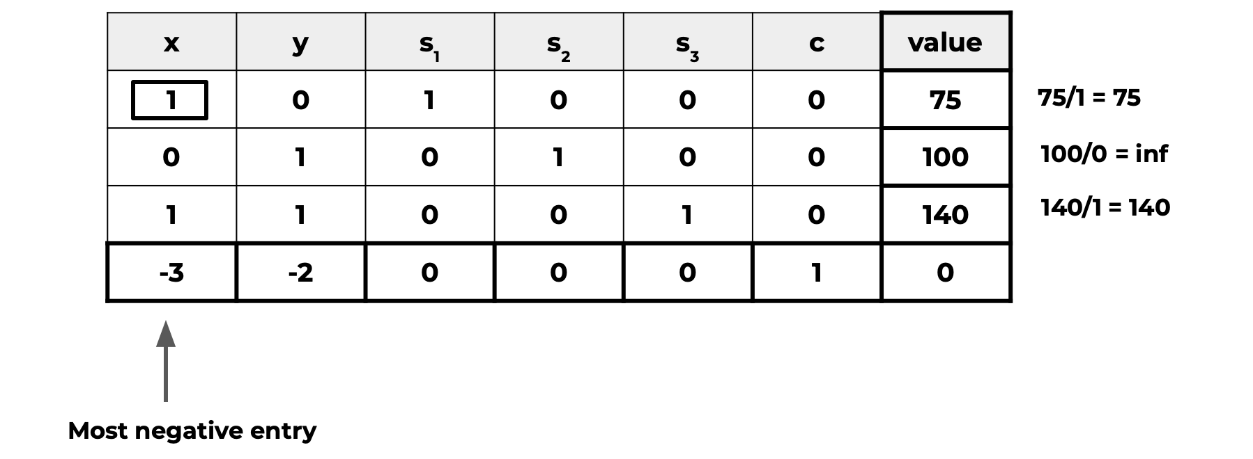
In this instance, our pivot column is x, **** called the entering variable, and the corresponding pivot row is the first one, R1, as it has the smallest quotient.
We choose the lowest value in the bottom row as it represents the lowest coefficient in the objective function. Therefore, optimizing for this column will increase the objective function the most.
Furthermore, we choose the row with the smallest quotient to not violate constraints. More information about why this is the case can be found here.
Step 4:
Using the pivot column, x, and row, R1, we want to make all entries in the pivot column 0 apart from R1. We do this by either adding or subtracting multiples of R1 with the other rows:

We see the new objective is 225, which corresponds to the (75,0) vertex in the plot we showed above. So, graphically we have moved from vertex (0,0) to vertex (75,0).
This step is essentially gaussian elimination.
Step 5:
Repeat steps 3 and 4 until all the entries in the last row (objective function) are non-zero:


Now, we have arrived at the optimal solution as there are no negatives in the bottom row. The optimal solution to our problem is then £355 when x = 75 and y = 65, in other words, the (75,65) vertex. This is the exact solution we found above using the graphical technique!
The algorithm steps themselves are not overly complicated, however, it can be tricky to understand what each step means. I have linked useful resources in the references section if you want to explore the simplex algorithm more and gain a deeper intuition behind the purpose of each step.
Other Algorithms
There are also more algorithms to solve LP problems. Below is a list with some provided links for the interested reader to check out:
- _Criss-cross algorithm_
- _[Interior point](https://en.wikipedia.org/wiki/Interior-point_method
- Ellipsoid algorithm
- Vaidya's algorithm
Linear Programming in Python
Fortunately, we don't have to do the simplex algorithm by hand when solving LP problems! In Python, two main packages do the heavy lifting for us:
I won't go into how to use them in this article but linked here is a great tutorial on applying these packages to your LP problem.
Summary & Further Thoughts
Linear programming (LP) is a very useful tool and can be applied to solve a wide range of problems, therefore is very useful for a Data Scientist to understand. The underlying concept behind LP is that it formulates the problem all in linear equations and inequalities enabling a quicker compute time. The most common method to solve LP problems is the simplex algorithm, which is luckily done for us in computing packages.
The full code used in this blog can be found on my GitHub here:
Medium-Articles/Optimisation/linear-programming at main · egorhowell/Medium-Articles
References & Further Reading
- Some more worked examples of simplex and graphical methods
- More mathematical deep dive into LP
- _A more in depth worked example of the simplex algorithm_
Another Thing!
I have a free newsletter, Dishing the Data, where I share weekly tips for becoming a better Data Scientist. There is no "fluff" or "clickbait," just pure actionable insights from a practicing Data Scientist.
