How to Train a Word2Vec Model from Scratch with Gensim

---

Word2Vec is a machine learning algorithm that allows you to create vector representations of words.

These representations, called embeddings, are used in many natural language processing tasks, such as word clustering, classification, and text generation.

---

The Word2Vec algorithm marked the beginning of an era in the NLP world when it was first introduced by Google in 2013.

It is based on word representations created by a neural network trained on very large data corpuses.

The output of Word2Vec are vectors, one for each word in the training dictionary, that effectively capture relationships between words.

Vectors that are close together in vector space have similar meanings based on context, and vectors that are far apart have different meanings. For example, the words "strong" and "mighty" would be close together while "strong" and "Paris" would be relatively far away within the vector space.

This is a significant improvement over the performance of the bag-of-words model, which is based on simply counting the tokens present in a textual data corpus.

In this article we will explore Gensim, a popular Python library for training text-based machine learning models, to train a Word2Vec model from scratch.

I will use the articles from my from my personal blog in Italian to act as a textual corpus for this project. Feel free to use whatever corpus you wish – the pipeline is extendable.

This approach is adaptable to any textual dataset. You'll be able to create the embeddings yourself and visualize them.

Let's begin!

Project requirements

Let's draw up a list of actions to do that serve as foundations of the project.

1. We'll create a new virtual environment (read here to understand how: How to Set Up a Development Environment for Machine Learning)

2. Install the dependencies, among which Gensim
3. Prepare our corpus to deliver to Word2Vec
4. Train the model and save it
5. Use TSNE and Plotly to visualize embeddings to visually understand the vector space generated by Word2Vec
6. BONUS: Use the Datapane library to create an interactive HTML report to share with whoever we want

By the end of the article we will have in our hands an excellent basis for developing more complex reasoning, such as clustering of embeddings and more.

I'll assume you've already configured your environment correctly, so I won't explain how to do it in this article. Let's start right away with downloading the blog data.

Dependencies

Before we begin let's make sure to install the following project level dependencies by running pip install XXXXX in the terminal.

• trafilatura
• pandas
• gensim
• nltk
• tqdm
• scikit-learn
• plotly
• datapane

We will also initialize a logger object to receive Gensim messages in the terminal.

Retrieve the corpus data

As mentioned we will use the articles of my personal blog in Italian (diariodiunanalista.it) for our corpus data.

Here is how it appears in Deepnote.

The textual data that we are going to use is under the article column. Let's see what a random text looks like

Regardless of language, this should be processed before being delivered to the Word2Vec model. We have to go and remove the Italian stopwords, clean up punctuation, numbers and other symbols. This will be the next step.

Preparation of the data corpus

The first thing to do is to import some fundamental dependencies for preprocessing.

# Text manipulation libraries
import re
import string
import nltk
from nltk.corpus import stopwords
# nltk.download('stopwords') <-- we run this command to download the stopwords in the project
# nltk.download('punkt') <-- essential for tokenization

stopwords.words("italian")[:10]
>>> ['ad', 'al', 'allo', 'ai', 'agli', 'all', 'agl', 'alla', 'alle', 'con']

Now let's create a preprocess_text function that takes some text as input and returns a clean version of it.

def preprocess_text(text: str, remove_stopwords: bool) -> str:
    """Function that cleans the input text by going to:
    - remove links
    - remove special characters
    - remove numbers
    - remove stopwords
    - convert to lowercase
    - remove excessive white spaces
    Arguments:
        text (str): text to clean
        remove_stopwords (bool): whether to remove stopwords
    Returns:
        str: cleaned text
    """
    # remove links
    text = re.sub(r"httpS+", "", text)
    # remove numbers and special characters
    text = re.sub("[^A-Za-z]+", " ", text)
    # remove stopwords
    if remove_stopwords:
        # 1. create tokens
        tokens = nltk.word_tokenize(text)
        # 2. check if it's a stopword
        tokens = [w.lower().strip() for w in tokens if not w.lower() in stopwords.words("italian")]
        # return a list of cleaned tokens
        return tokens

Let's apply this function to the Pandas dataframe by using a lambda function with .apply.

df["cleaned"] = df.article.apply(
    lambda x: preprocess_text(x, remove_stopwords=True)
  )

We get a clean series.

Let's examine a text to see the effect of our preprocessing.

The text now appears to be ready to be processed by Gensim. Let's carry on.

Word2Vec training

The first thing to do is create a variable texts that will contain our texts.

texts = df.cleaned.tolist()

We are now ready to train the model. Word2Vec can accept many parameters, but let's not worry about that for now. Training the model is straightforward, and requires one line of code.

from gensim.models import Word2Vec

model = Word2Vec(sentences=texts)

Our model is ready and the embeddings have been created. To test this, let's try to find the vector for the word overfitting.

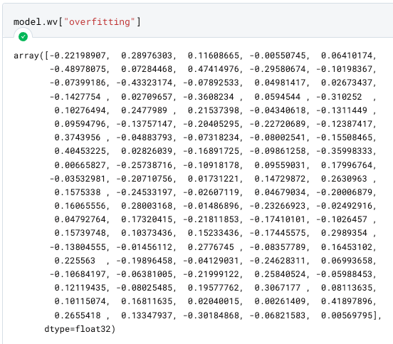
By default, Word2Vec creates 100-dimensional vectors. This parameter can be changed, along with many others, when we instantiate the class. In any case, the more dimensions associated with a word, the more information the neural network will have about the word itself and its relationship to the others.

Obviously this has a higher computational and memory cost.

Please note: one of the most important limitations of Word2Vec is the inability to generate vectors for words not present in the vocabulary (called OOV – out of vocabulary words).

To handle new words, therefore, we'll have to either train a new model or add vectors manually.

Calculate the similarity between two words

With the cosine similarity we can calculate how far apart the vectors are in space.

With the command below we instruct Gensim to find the first 3 words most similar to overfitting

model.wv.most_similar(positive=['overfitting'], topn=3))

Let's see how the word "when" (quando in Italian) __ is present in this result. It will be appropriate to include similar adverbs in the stop words to clean up the results.

To save the model, just do model.save("./path/to/model").

Visualize embeddings with TSNE and Plotly

Our vectors are 100-dimensional. It's a problem to visualize them unless we do something to reduce their dimensionality.

We will use the TSNE, a technique to reduce the dimensionality of the vectors and create two components, one for the X axis and one for the Y axis on a scatterplot.

In the .gif below you can see the words embedded in the space thanks to the Plotly features.

Here is the code to generate this image.

def reduce_dimensions(model):
    num_components = 2  # number of dimensions to keep after compression

    # extract vocabulary from model and vectors in order to associate them in the graph
    vectors = np.asarray(model.wv.vectors)
    labels = np.asarray(model.wv.index_to_key)  

    # apply TSNE 
    tsne = TSNE(n_components=num_components, random_state=0)
    vectors = tsne.fit_transform(vectors)

    x_vals = [v[0] for v in vectors]
    y_vals = [v[1] for v in vectors]
    return x_vals, y_vals, labels

def plot_embeddings(x_vals, y_vals, labels):
    import plotly.graph_objs as go
    fig = go.Figure()
    trace = go.Scatter(x=x_vals, y=y_vals, mode='markers', text=labels)
    fig.add_trace(trace)
    fig.update_layout(title="Word2Vec - Visualizzazione embedding con TSNE")
    fig.show()
    return fig

x_vals, y_vals, labels = reduce_dimensions(model)

plot = plot_embeddings(x_vals, y_vals, labels)

This visualization can be useful for noticing semantic and syntactic tendencies in your data.

For example, it's very useful for pointing out anomalies, such as groups of words that tend to clump together for some reason.

Parameters of Word2Vec

By checking on the Gensim website we see that there are many parameters that Word2Vec accepts. The most important ones are vectors_size, min_count, window and sg.

• vectors_size : defines the dimensions of our vector space.
• min_count: Words below the min_count frequency are removed from the vocabulary before training.
• window: maximum distance between the current and the expected word within a sentence.
• sg: defines the training algorithm. 0 = CBOW (continuous bag of words), 1 = Skip-Gram.

We won't go into detail on each of these. I suggest the interested reader to take a look at the Gensim documentation.

Let's try to retrain our model with the following parameters

VECTOR_SIZE = 100
MIN_COUNT = 5
WINDOW = 3
SG = 1

new_model = Word2Vec(
    sentences=texts, 
    vector_size=VECTOR_SIZE, 
    min_count=MIN_COUNT, 
    sg=SG
)

x_vals, y_vals, labels = reduce_dimensions(new_model)

plot = plot_embeddings(x_vals, y_vals, labels)

The representation changes a lot. The number of vectors is the same as before (Word2Vec defaults to 100), while min_count, window and sg have been changed from their defaults.

I suggest to the reader to change these parameters in order to understand which representation is more suitable for his own case.

BONUS: Create an interactive report with Datapane

We have reached the end of the article. We conclude the project by creating an interactive report in HTML with Datapane, which will allow the user to view the graph previously created with Plotly directly in the browser.

This is the Python code

import datapane as dp

app = dp.App(
    dp.Text(text='# Visualizzazione degli embedding creati con Word2Vec'),
    dp.Divider(),
    dp.Text(text='## Grafico a dispersione'),
    dp.Group(
        dp.Plot(plot),
        columns=1,
    ),
)
app.save(path="test.html")

Datapane is highly customizable. I advise the reader to study the documentation to integrate aesthetics and other features.

Conclusion

We have seen how to build embeddings from scratch using Gensim and Word2Vec. This is very simple to do if you have a structured dataset and if you know the Gensim API.

With embeddings we can really do many things, for example

• do document clustering, displaying these clusters in vector space
• research similarities between words
• use embeddings as features in a Machine Learning model
• lay the foundations for machine translation

and so on. If you are interested in a topic that extends the one covered here, leave a comment and let me know

Tags: Gensim Machine Learning NLP Python Word2vec

Comment