Isochrones in Python
In geospatial sciences and location intelligence, isochrones represent geographical areas that can be reached within a certain amount of time from a specific point. For instance, in the context of walking distances, isochrones are helpful tools in the tool of professionals like urban planners aiming to understand accessibility and connectivity within a given area.
By visualizing isochrones, Data Science can provide a quick and easy-to-use tool to help gaining insights into the level of connectivity and walking accessibility of neighborhoods, help to identify areas that are well-connected, and pinpoint potential areas of infrastructural improvements.
Further, in this article, we will provide an overview of how to generate walking distance isochrones using the Python packages NetworkX (designed for graph analytics) and OSMNnx (combining OpenStreetMap and NetworkX) while using a randomly selected district of Budapest, District 12, as an example. First, we download the road network of the area, then pick a random node (a random intersection) in it, and then draw the 5, 10, 20 and 30 minutes walking isochrones around it.
All images were created by the author.
Data acquisition
First, let's import OSMnx, and use it to download the administrative boundaries of the target area. In this example, we use District 12 of Budapest. However, this can be replaced by any place name you prefer, which you can easily browse on OpenStreetMap. Then, we further use OSMnx to download the road network of the target area and output the size of this node network in terms of the number of road intersections and segments. Additionally, we need to specify the type of network, which is now set to ‘walk' to get only the walkable parts of the road network.
Python"># Importing osmnx
import osmnx as ox

# Define the polygon for the 1st district of Budapest
admin_district = ox.geocode_to_gdf('12th district, Budapest')
admin_district.plot()
admin_poly = admin_district.geometry.values[0]

# Load the graph from OSMnx
G = ox.graph_from_polygon(admin_poly, network_type='walk')

print('Number of intersections: ', G.number_of_nodes())
print('Number of road segments:',  G.number_of_edges())
The output:

Reachability polygons
Now, let's build the walkability isochrone polygons. For this, first, we assume an average walking speed of 5 km/h (1.39 m/s), and use this walking speed to attach a walking time to each edge of the road network. Then, we pick a random node to start from, and define the list of walkability ranges: 5, 10, 20, and 30 minutes.
# Define the walking speed (5 km/h -> 1.39 m/s)
walking_speed = 1.39 # in meters per second
# Calculate travel time for each edge
for u, v, data in G.edges(data=True):
# Calculate travel time in seconds
data['travel_time'] = data['length'] / walking_speed
# Pick a center node
center_node = list(G.nodes())[30] # starting point
# Generate isochrones
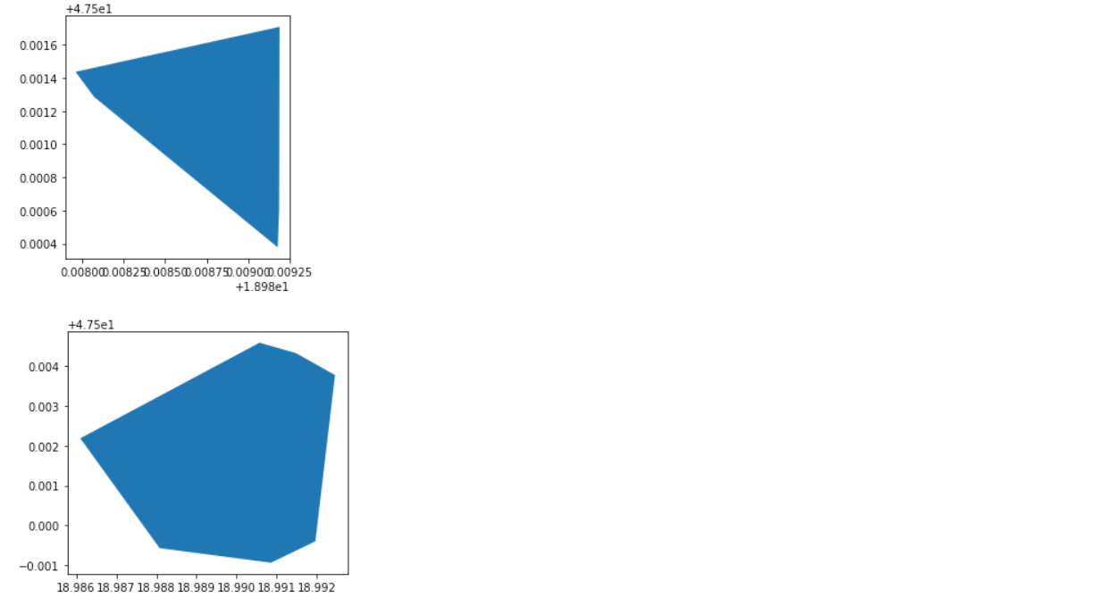
isochrone_times = [5, 10, 20, 30] # isochrones in minutesTo create the reachability polygons, first we use use the built-in function of NetworkX called _egograph which returns a particular subgraph of the original road network which contains all nodes within a given radius, according to any distance metrics of our choosing. If we pick _traveltime, we can already return the subgraph reachable within a given amount oftime and store this as an edge attribute we call _traveltime.
Then, we need to extract all the node coordinates of this subgraph, which we will store in the list _nodepoints. As a final step, we turn these into a polygon, plot it, and save it for the next section.
# Library imports
import networkx as nx
from shapely.geometry import Point, Polygon
import geopandas as gpd

isochrone_polys = []

for time in isochrone_times:
    subgraph = nx.ego_graph(G,
                            center_node,
                            radius=time*60,
                            distance='travel_time')

    node_points = [Point((data['x'], data['y']))
                   for node, data in subgraph.nodes(data=True)]

    polygon = Polygon(gpd.GeoSeries(node_points).unary_union.convex_hull)
    gpd.GeoDataFrame([polygon], columns = ['geometry']).plot()
    isochrone_polys.append(gpd.GeoSeries([polygon]))
The output – all the walkability isochrone polygons, for 5, 10, 20, and 30 minutes, respectively:

Visualizing the isochrones
Finally, let's use Matplotlib and red-to-green coloring to plot and visualize the isochrones above the road network.
# import plotting libs
import matplotlib.pyplot as plt
import matplotlib.patches as mpatches

# Create visuals
fig, ax = plt.subplots(figsize=(8, 8))

# Define the colors of the isochrones
colors = ['red', 'orange', 'yellow', 'green']

# Plot the isochrones
for idx, (polygon, time) in
    enumerate(reversed(list(zip(isochrone_polys, isochrone_times)))):
    polygon.plot(ax=ax, color=colors[idx], alpha=0.4, label=f'{time} min')
    polygon.plot(ax=ax, color = 'none', edgecolor = colors[idx], linewidth = 3)

# Manually create legend handles
handles = [
    mpatches.Patch(color=colors[idx], alpha=0.6, label=f'{time} min')
    for idx, time in enumerate(reversed(isochrone_times))
]

# Plot the network
ox.plot_graph(G, ax=ax, node_size=0, edge_linewidth=0.7, show=False)

# Add the legend to the plot and set the title
ax.set_title('Isochrones in Budapest District 12', fontsize=16)
legend = plt.legend(handles=handles)
legend.get_frame().set_linewidth(0)  # Remove the legend box's frame

# Show the plot
plt.show()
Conclusion
In this article, we reviewed how to generate so-called walkability isochrones – polygon areas which highlight the area reachable from a starting location within a given amount of time. While this concept is a really intersting use of spatial networks, it is of even higher importance in Urban Planning, when computing the range of attraction of critical public services or quantifying the accessiblity of amenities within areas.
In case you would like to read more on spatial networks and further advance your geospatial Python skills, check out my brand new book, Geospatial Data Science Essentials – 101 Practical Python Tips and Tricks!
