Matrix Approximation in Data Streams

Author:Murphy | View: 20924 | Time: 2025-03-23 12:40:14

Matrix approximation is a heavily studied sub-field in data mining and Machine Learning. A large set of data analysis tasks rely on obtaining a low rank approximation **** of matrices. Examples are dimensionality reduction, anomaly detection, data de-noising, clustering, and recommendation systems. In this article, we look into the problem of matrix approximation, and how to compute it when the whole data is not available at hand!

The content of this article is partly taken from my lecture at Stanford -CS246 course. I hope you find it useful. Please find the full content here.

Data as a matrix

Most data generated on web can be represented as a matrix, where each row of the matrix is a data point. For example, in routers every packet sent across the network is a data point that can be represented as a row in a matrix of all data points. In retail, every purchase made is a row in the matrix of all transactions.

At the same time, almost all data generated over web is of a streaming nature; meaning the data is generated by an external source at a rapid rate which we have no control over. Think of all searches users make on Google search engine in a every second. We call this data the streaming data; because just like a stream it pours in.

Some examples of typical streaming web-scale data are as following:

Figure 2: Size of typical streaming web-scale data – Image by the author

Think of streaming data as a matrix A containing n rows in d-dimensional space, where typically n >> d. Often n is in order of billions and increasing.

Data streaming model

In streaming model, data arrives at high speed, one row at a time, and algorithms must process the items fast, or they are lost forever.

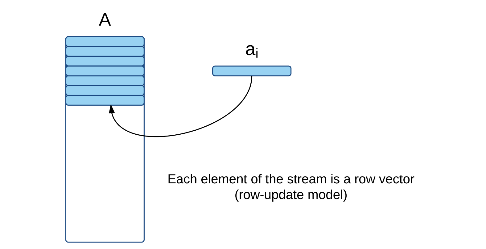
In data streaming model, algorithms can only make one pass over the data and they work with a small memory to do their processing.

Rank-k approximation

Rank-k approximation of a matrix A is a smaller matrix B of rank k such that B approximates A accurately. Figure 2 demonstrates this notion.

Figure 4: Getting a much smaller sketch B from A – Image by the author

B is often called a sketch of A. Note, in data streaming model, B will be much smaller than A such that it fits in memory. In addition, rank(B) << rank(A). For example, if A is a term-document matrix with 10 billion documents and 1 million words then B would probably be a 1000 by million matrix; i.e. 10 million times less rows!

The rank-k approximation has to approximate A "accurately". While accurately is a vague notion, we can quantify it via various error definitions:

1️⃣ Covariance error:

The covariance error is the Frobenius norm or L2 norm of differences between covariance of A and covariance of B. This error is mathematically defined as following:

covariance error definition – Image by the author

2️⃣ Projection error:

The projection error is the norm of the residual when data points in A are projected onto the subspace of B. This residual norm is measured as either L2 norm or Frobenius norm:

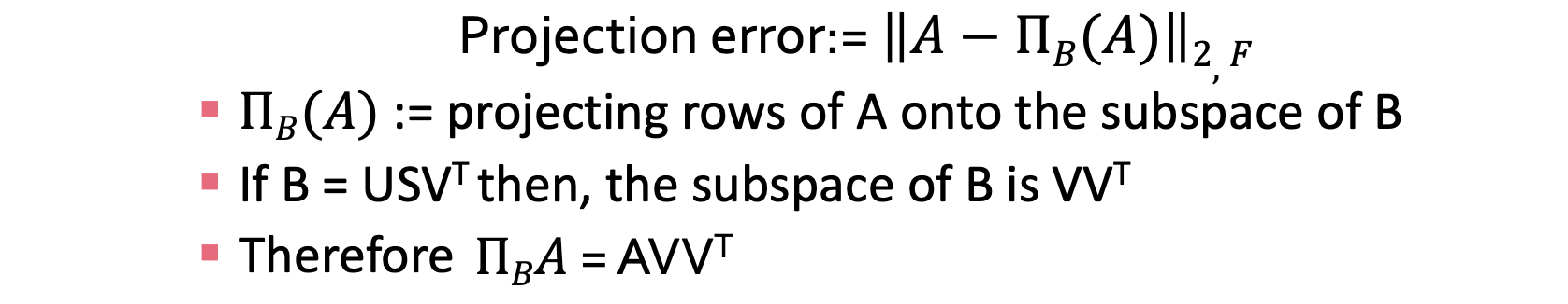
projection error definition – Image by the author

These errors assess the quality of the approximation; the smaller they are the better the approximation is. But how small can they be?

When we compute these errors, we must have a baseline to compare them against. The baseline, everyone uses in field of matrix sketching is the rank-k approximation created by Singular Value Decomposition (SVD)! SVD computes the best rank-k approximation! Meaning it causes the smallest error on both "covariance error" and "projection error".

The best rank-k approximation to A is denoted as Aₖ. Therefore, the least error caused by SVD is :

least rank k approximation error – Image by the author

SVD, decomposes a matrix A into three matrices:

The left singular matrix U
The singular values matrix S
The right singular matrix V

U and V are orthonormal, meaning that their columns are of unit norm and they are orthogonal; i.e. the dot product of every two columns in U (similarly in V) is zero. The matrix S is diagonal; only entries on the diagonal are non-zeros and they are sorted in descending order.

Figure 5: Singular value decomposition – Image by the author

SVD computes the best rank-k approximation by taking the first k columns of U and V and the first k entries of S:

Figure 6: Rank k approximation by SVD – Image by the author

As we mentioned, the Aₖ computed in this way has the lowest approximation error among any matrices B with rank k or lower. However, SVD is a very time-consuming method, it requires runtime O(nd²) if A is n-by-d, and it is not applicable to matrices in data streaming fashion. In addition, SVD is not efficient for sparse matrices; it does not utilize sparsity of the matrix in computing approximation.

❓Now the question is how do we compute matrix approximation in streaming fashion ?

There are three main family of methods in streaming matrix approximations:

1️⃣ Row sampling based

2️⃣ Random projection based

3️⃣ Iterative sketching

Row sampling based methods

These methods sample a subset of "important" rows with respect to a well-defined probability distribution. These methods differ is in how they define the notion of "importance". The generic framework is that they construct the sketch B as following:

They first assign a probability to each row in the streaming matrix A
Then they sample l rows from A (often with replacement) to construct B
Lastly, they rescale B appropriately to make it an unbiased estimate of A

Figure 7: Row sampling with replacement to build sketch B – Image by the author

Note, the probability assigned to rows in step 1, is in fact the "importance" of the row. Think of "importance" of an item as the weight associated to the item e.g. for file records, the weight can be size of the files. Or for IP addresses, the weight can be the number of times the IP address makes a request.

In matrices, each item is a row vector, and its weight is the squared of its norm; also called L2 norm. There is a row sampling algorithm that samples with respect to L2 norm of rows in a one pass over data. This algorithm is called "L2-norm row sampling", and its pseudocode is as following:

Figure 8: L2-norm row sampling algorithm – Image by the author

This algorithm samples l = O(k/ε²) rows with replacement and achieves the following error bound:

Figure 9: Error guarantee of L2-norm row sampling – Image by the author

Note, this is a weak error bound, as it is bounded by total Frobenius norm of A, which can be a large number! There is an extension of this algorithm that performs better; let's take a look at it.

Extension: There is a variation of this algorithm that samples both rows and columns! It is called "CUR" algorithm and it performs better than "L2-norm row sampling" method. The CUR method creates three matrices C, U and R by sampling rows and columns of A. Here is how it works:

Step 1: CUR first samples few columns of A, each with the probability proportional to the norm of the columns. This makes the matrix C.

Figure 10: CUR algorithm step 1— Image by the author

Step 2: Then CUR samples few rows of A, each with probability proportional to the norm of the rows. This forms matrix R.

Step 3: The CUR then computes the pseudo-inverse of the intersection of C and R. This is called matrix U.

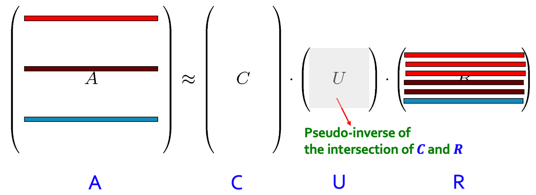
Figure 11: CUR algorithm step 2,3— Image by the author

Finally, the product of these three matrices, i.e. C.U.R approximates A, and provides a low-rank approximation. This algorithm achieves the following error bound sampling l = O(k log k/ε²) rows and columns.

Figure 12: CUR Error guarantee – Image by the author

Note, how this is a much tighter bound as compared to L2-norm row sampling.

Summary: The row sampling family of methods (CUR included) samples rows (and columns) to form a low-rank approximation; therefore they are very intuitive and form interpretable approximations.

In the next section, we see another family of methods that are data oblivious.

Random projection based methods

The key idea of these group of methods is that if points in a vector space are projected onto a randomly selected subspace of suitably high dimension, then the distances between points are approximately preserved.

Johnson-Lindenstrauss Transform (JLT) specifies this nicely as following: d datapoints in any dimension (e.g. n-dimensional space for n≫d) can get embedded into roughly log d dimensional space, such that their pair-wise distances are preserved to some extent.

A more precise and mathematical definition of JLT is as following:

Figure 13: JLT definition – Image by the author

There are many ways to construct a matrix S that preserve pair-wise distances. All such matrices are called to have the JLT property. The image below, shows few well-known ways of creating such matrix S:

One simple construction of S, as shown above, is to pick entries of S to be independent random variables drawn from N(0,1), and rescale S by √(1/r):

Figure 14: JLT matrix – Image by the author

This matrix has the JLT property [6], and we use it to design a random projection method as following:

Figure 15: Random projection method – Image by the author

Note the second step, projects data points from a high n-dimensional space into a lower r-dimensional space. It's easy to show [6]that this method produces an unbiased sketch:

Figure 16: Random projection provides an unbiased approximation— Image by the author

The random projection method achieves the following error guarantee if it sets r = O(k/ε + k log k). Note that they achieve better bound than row sampling methods.

Figure 17: Random projection error bound— Image by the author

There is a similar line of work to random projection that achieves better time bound. It is called Hashing techniques [5]. This method take a matrix S which has only one non-zero entries per column and that entry is either 1 or -1. They compute the approximation as B = SA.

Summary: Random projection methods are computationally efficient, and are data oblivious as their computation involves only a random matrix S. Compare it to row sampling methods that need to access data to form a sketch.

Iterative Sketching

These methods work over a stream A= where each item is read once, get processed quickly and not read again. Upon reading each item, they update the sketch B.

State of the art method in this group is called "Frequent Directions", and it is based on Misra-Gries algorithm for finding frequent items in a data stream. In what follows, we first see how Misra-Gries algorithm for finding frequent items work, then we extend it to matrices.

Misra-Gries algorithm for finding frequent items

Suppose there is a stream of items, and we want to find frequency f(i) of each item.

Figure 19: frequent item counting over streams – Image by the author

If we keep d counters, we can count frequency of every item. But it's not good enough as for certain domains such IP addresses, queries, etc. the number of unique items are way too many.