Summer Olympic Games Through the Lens of Data

This year's Summer Olympic Games, held in Paris, is upon us in a few days, so I decided to dive into the history of the Olympics as a data scientist, otherwise not too deeply vested in the details of Olympic sports, would do.

Namely, relying on public Wikipedia data, I wanted to figure out which countries have been the biggest stars of the Olympics before and who are the biggest competitors of each other. In particular, I collected the total number of Gold, Silver, and Bronze medals won by each country, broken down to the level of individual sports. Then, I put the total number of medals on global Maps, using the medal-sport profiles to build and visualize a similar network of countries, illustrating the competing clusters of countries with similar sports profiles.

Let's get started by building the data set!

All images were created by the author.

1. Database

1. 1. Getting the complete list olympic countries

First, I went after the Wikipedia site titled All-time Olympic Games medal table, which has a short summary of each country's Olympic performance history, including reference links pointing to the detailed history of each country. First, I extract these URLs pointing to the detailed profile of each country as follows:

# libraries needed for the scraping
import requests
from bs4 import BeautifulSoup
import re

# the source urls
url = 'https://en.wikipedia.org/wiki/All-time_Olympic_Games_medal_table'

# Send a request to the website and get the HTML content
response = requests.get(url)
html_content = response.content

# Parse the HTML content using BeautifulSoup
soup = BeautifulSoup(html_content, 'html.parser')

# Find all  tags with the specific URL pattern which matches country-level sites
pattern = re.compile(r'/wiki/[^"]+_at_the_Olympics')

# Extract the URLs
urls = []
for a_tag in soup.find_all('a', href=pattern):
    url = a_tag['href']
    urls.append('https://en.wikipedia.org' + url)
urls = sorted(list(set(urls)))
print('Number of urls:' , len(urls))   

# Print the extracted URLs
for url in urls[0:10]:
    print(url)

The number of country-level urls and the first ten examples of those:

1.2. Downloading the number of medals per country

Now, let's use these country-level URLs to download each country's summary medal profile first. As an illustration, let's see what the profile of Greece looks like . We can see that out of the total 121 meals, there were 35 gold, 45 silver, and 41 bronze.

Now, let's download the summary profiles of all countries and then show what the summary profiles look like.

countries_medals = {}

for idx, url in enumerate(urls):

    # Get teh country's name
    country = url.split('/')[-1].split('_at')[0]  

    # Send a request to the website and get the HTML content
    response = requests.get(url)
    html_content = response.content

    # Parse the HTML content using BeautifulSoup
    soup = BeautifulSoup(html_content, 'html.parser')

    # Extract the medal counts
    medals = {}
    for dt, dd in zip(soup.find_all('dt'), soup.find_all('dd')):
        medal_type = dt.text.strip()
        try:
            count = int(dd.text.strip())
            medals[medal_type] = count
        except:
            pass

    # Save the medal data
    countries_medals[country] = medals

# re-oreganize and show the results
countries_medals_winners = {c : medals for c, medals in countries_medals.items() if 'Total' in medals and medals['Total'] > 0}
print(len(countries_medals_winners))

from itertools import islice
dict(islice(countries_medals_winners.items(), 5))  

The output of this cell shows that 154 countries have won at least one medal and the first five example country profiles of these.

1.3. Get the sport – medals profile for an example country

Now that we have the summary profile of each country – to be used later in this article -it is time to take a closer look at the sport-level breakdown of these results. Again, let's see what that looks like for Greece on Wikipedia:

Now, let's collect these data using Python. An early warning – some countries will be more problematic and will throw errors, so I will collect them into a dedicated list. Besides, I will also test if the total number of medals coming from the initial profile and coming from the sport-level breakdown are matching or not.

import pandas as pd
countries_profiles = {}
mismatch_errors = {}
errors = []

for url in urls:

    try:

        # Check if the country has medals
        country = url.split('/')[-1].split('_at')[0]
        if country in countries_medals_winners:

            # Send a request to the website and get the HTML content
            response = requests.get(url)
            html_content = response.content

            # Parse the HTML content using BeautifulSoup
            soup = BeautifulSoup(html_content, 'html.parser')
            tables = soup.find_all('table', {'class': 'wikitable'})

            for table in tables:

                if 'sport' in table.text.lower():   

                    # Extract table headers
                    headers = []
                    for th in table.find_all('th'):
                        headers.append(th.get_text(strip=True))

                    # Create the sport profile DF
                    data = []
                    headers = headers[0:5]
                    headers[0] = 'Sport'
                    print(headers)
                    for tr in table.find_all('tr')[1:-1]:
                        cells = tr.find_all(['td', 'th'])
                        row = [cell.get_text(strip=True) for cell in cells]
                        row = [row[0]] + [int(r) for r in row[1:]]

                        if len(row)>0:
                            data.append({h : row[idx] for idx, h in enumerate(headers)})

                    df_profile = pd.DataFrame(data)
                    df_profile = df_profile.set_index('Sport')

                    #display(df_profile)
                    countries_profiles[country] = df_profile

                    print(country)
                    print('Number of medals from the summary pages: ', countries_medals_winners[country]['Total'])
                    print('Number of medals from the sport profile: ', df_profile['Total'].sum())
                    if countries_medals_winners[country]['Total'] != df_profile['Total'].sum():
                        print('MEDAL COUNT MISMATCH ERROR')
                        mismatch_errors[country] = url
                    print()
                    break  

    except:
        print('ERROR: ', country, url)
        errors.append((country, url))
        pass

A sample of this cell's output:

The summary statistics of this data collection step:

print('Number of medal-winning countries', len(countries_medals_winners))
print()
print('Results in collecting country-level sport medal profiles:')
print('Number of errors: ', len(errors))
print('Number of mismatches: ', len(mismatch_errors))

Here, we can see that there are seven errors – countries that have Olympic medals, but my script was unable to collect their profile. Let's clean this up in the next section.

1.4. Clean the sport-level medal profiles erros

First, let's print all the problematic country-level urls with direct errors:

for err in errors:
    print(err[0], err[1], countries_medals_winners[err[0]]['Total'])

As for the errors, we can see from the URLs that only 4 out of the 7 are actual countries. Then, when clicking on the URLs, we quickly learn that Egypt and Estonia simply do not have that type of tabel information on their Wiki. Then, it also turns out that while India and Pakistan have that in some ways, their site is completelydifferently structured than the rest.

At this point, if this was a serious consulting or research project, I would maybe write scripts for each of them separately.However, now we just want to see cool and reliable maps without any risking shareholder value; I just ask ChatGPT to gather this information and output it in the following data structures. This is also an excellent example of how a streamlined, well-maintained data source, like Wikipedia, can play a trick on us, which highlights the importance of robustness and data cleaning in data processing pipelines. Let's add the ChatGPT-based clean-up data:

# Define the dictionaries for each country
egypt_medals = {
    'Swimming': {'Gold': 2, 'Silver': 4, 'Bronze': 1, 'Total': 7},
    'Field hockey': {'Gold': 1, 'Silver': 0, 'Bronze': 0, 'Total': 1}
}

estonia_medals = {
    'Swimming': {'Gold': 2, 'Silver': 4, 'Bronze': 1, 'Total': 7},
    'Field hockey': {'Gold': 1, 'Silver': 0, 'Bronze': 0, 'Total': 1}
}

pakistan_medals = {
    'Swimming': {'Gold': 2, 'Silver': 4, 'Bronze': 1, 'Total': 7},
    'Field hockey': {'Gold': 1, 'Silver': 0, 'Bronze': 0, 'Total': 1}
}

india_medals = {
    'Swimming': {'Gold': 2, 'Silver': 4, 'Bronze': 1, 'Total': 7},
    'Field hockey': {'Gold': 1, 'Silver': 0, 'Bronze': 0, 'Total': 1}
}

# Convert each dictionary to a DataFrame
countries_profiles['Egypt'] = pd.DataFrame.from_dict(egypt_medals, orient='index').rename_axis('Sport')
countries_profiles['Estonia'] = pd.DataFrame.from_dict(estonia_medals, orient='index').rename_axis('Sport')
countries_profiles['Pakistan'] = pd.DataFrame.from_dict(pakistan_medals, orient='index').rename_axis('Sport')
countries_profiles['India'] = pd.DataFrame.from_dict(india_medals, orient='index').rename_axis('Sport')

1.5. Clean the sport-profile-level medal count mismatch erros

Now also see the medal-number mismatch errors:

for country, url in mismatch_errors.items():
    print(url)

After cleaning through a dozen examples, my conclusion was that the main differences come from the fact that not all tables solely contain the summer game medals. So, the next task was to collect all summer sports and filter all medal profiles to be restricted to the summer medal profiles only.

First, I manually combined Wikipedia and ChatGPT, collected the list of summer sports, and then cleaned up the dictionaries. As the following code block shows, this resulted in 35 different sports covering the entire history of the Summer Olympics Games.

summer_olympic_sports = [
    'Archery',
    'Athletics',
    'Badminton',
    'Baseball',
    'Softball',
    'Basketball',
    'Boxing',
    'Canoeing',
    'Cycling',
    'Diving',
    'Equestrian',
    'Fencing',
    'Field hockey',
    'Football',
    'Golf',
    'Gymnastics',
    'Handball',
    'Judo',
    'Karate',
    'Modern pentathlon',
    'Rowing',
    'Rugby sevens',
    'Sailing',
    'Shooting',
    'Skateboarding',
    'Sport climbing',
    'Surfing',
    'Swimming',
    'Table tennis',
    'Taekwondo',
    'Tennis',
    'Triathlon',
    'Volleyball',
    'Weightlifting',
    'Wrestling'
]

print(' Number of summer sports: ', len(set(summer_olympic_sports)), 'n',
      'Number of sports in the Wiki data: ', len(set(all_sports)), 'n',
      'Their overlap: ', len(set(summer_olympic_sports).intersection(set(all_sports))))

countries_profiles_clean = {}
for country, profile in countries_profiles.items():
    if 'Gold' in profile.keys():
        countries_profiles_clean[country.replace('_', ' ')] = profile[profile.index.isin(summer_olympic_sports)]

countries_medals_winners_summer = {}
for country, profile in countries_profiles_clean.items():
    total_d = profile.sum().to_dict()
    total_d= {k : v for k, v in total_d.items() if k in ['Gold', 'Silver', 'Bronze', 'Total']}
    countries_medals_winners_summer[country] = total_d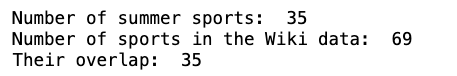        

By the end of this step, we officially arrived at the end of the rather tedious data collecting and cleaning process – now we can get the fun stuff going on with the analytics and visualization parts.

2. Analytics

2.1 Top Olimpic countries

First, let's do some basic stats on the data set we created – display the top 10 most prolific countries in terms of the total number of medals, and plot the golden countries – the top 10 countries with the highest number of gold medals.

df_summary = pd.DataFrame(countries_medals_winners_summer).T
df_summary.index = [i.replace('_', ' ') for i in list(df_summary.index)]
df_summary.sort_values(by = 'Total', ascending = False).head(10)

df_summary.sort_values(by = 'Gold', ascending = False).head(10)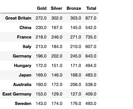

These two lists show that Great Britain and France seem to be ruling the Olympics, while China is the best in terms of the relative number of gold. Let's explore these correlations a little further.

2.2. Country-level features, correlations

To incorporate this dimension, first, I import a world map, stored as a built-in data set of GeoPandas, sourced from Natural Earth. (Note: the latest version of GeoPandas doesn't have it, so I added my version here as well). This data set contains both the geographical boundaries of each country as polygons and estimated population and GDP levels, which we can contrast to the medal statistics.

Then, I cleaned some country names to match the Wikipedia-based country names to the Natural Earth ones. Additionally, here I will focus on countries with at least ten medals in total, to make the semi-manual name matching a little easier.

import geopandas as gpd
print(gpd.__version__)

# parse the country-level data table
world = gpd.read_file(gpd.datasets.get_path('naturalearth_lowres'))
display(world.head())

# test the country name lists of the Wiki and Natural Earth data sets
countries_1 = set(world.name)
countries_2 = set(df_summary[df_summary.Total>9].index)
print(len(countries_1), len(countries_2), len(countries_1.intersection(countries_2)))
print('Country name mismatches:')
print(countries_2.difference(countries_1))

# country name clean-up
matches = {
    'Chinese Taipei': 'Taiwan',
    'Czech Republic': 'Czechia',
    'Dominican Republic': 'Dominican Rep.',
    'Great Britain': 'United Kingdom',
}

for v1, v2 in matches.items():
    world.name = world.name.str.replace(v2, v1)

df_merged = df_summary.merge(world, left_index = True, right_on = 'name')
df_merged.head()

The output of this code block:

Now all we have left is to compute the correlation matrix of the country-level features:

df_merged.corr()

It looks that in general, the number of Gold, Silver, and Bronze medals are really highly correlated, implying that there isn't really any golden nation who always wins, but rather implying a by-chance nature of how the medals get distributed – however, to say this for certain, further statistical tests will be needed.

Interestingly, though, we see a really low (0.25) correlation between the number of medals of any sort and a country's population. One may expect that sports are fair – and the larger the pool of potential top athletes, the better the chances to excel at different sports. This may be true for one or two sports per country; however, the general trend shows that instead of population, it is money – expressed by GDP estimates – that drives Olympic success.

2.3. Olympic maps

Now, let's use the combined map of geographical data and medal information and create Olympic maps showing each country's color based on the number of gold, silver, and bronze medals they have won. For this, we rely on GeoPandas' plotting capabilities combined with Matplotlib.

First, let's create appropriate color maps for the three types of medals.

import matplotlib.pyplot as plt
import numpy as np
from matplotlib.colors import LinearSegmentedColormap

# Define the colors for the gradients
colors_gold = ["#FFFFFF", "#FFD700"]  # White to Gold
colors_silver = ["#FFFFFF", "#C0C0C0"]  # White to Silver
colors_bronze = ["#FFFFFF", "#CD7F32"]  # White to Bronze

# Create the colormaps
cmap_gold = LinearSegmentedColormap.from_list("WhiteToGold", colors_gold)
cmap_silver = LinearSegmentedColormap.from_list("WhiteToSilver", colors_silver)
cmap_bronze = LinearSegmentedColormap.from_list("WhiteToBronze", colors_bronze)

# Create a gradient image
gradient = np.linspace(0, 1, 256)
gradient = np.vstack((gradient, gradient))

# Plot the gradients
fig, axes = plt.subplots(nrows=3, figsize=(6, 6))

axes[0].imshow(gradient, aspect='auto', cmap=cmap_gold)
axes[0].set_title('White to Gold')
axes[0].axis('off')

axes[1].imshow(gradient, aspect='auto', cmap=cmap_silver)
axes[1].set_title('White to Silver')
axes[1].axis('off')

axes[2].imshow(gradient, aspect='auto', cmap=cmap_bronze)
axes[2].set_title('White to Bronze')
axes[2].axis('off')

plt.tight_layout()
plt.show()

Next, turn the merged geospatial data into a visually appealing map projection, the Mollweidwe projection system:

gdf_merged = gpd.GeoDataFrame(df_merged)
gdf_merged.crs = 4326
gdf_merged = gdf_merged.to_crs('ESRI:54009')

Then, do the maps:

f, ax = plt.subplots(1,1,figsize=(12,4))
gdf_merged.plot(column = 'Gold', ax=ax, cmap = cmap_gold, edgecolor = 'w', linewidth = 0, legend = True)

ax.set_title('Number of Gold medals per country', fontsize = 17, pad = 20)
ax.get_xaxis().set_visible(False)
ax.get_yaxis().set_visible(False)

fig.patch.set_facecolor('#2f2f2f')
ax.set_facecolor('#2f2f2f')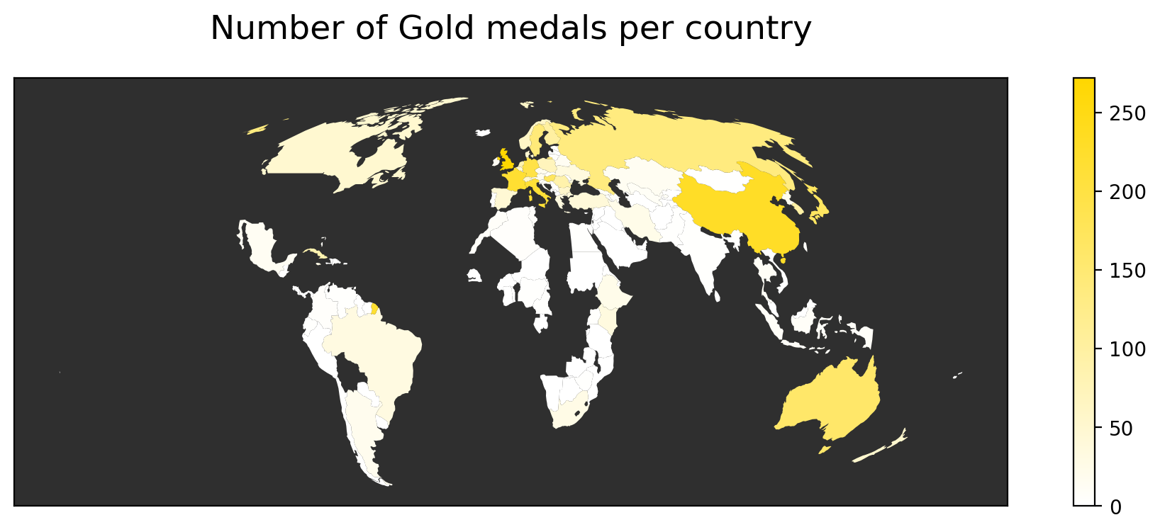

f, ax = plt.subplots(1,1,figsize=(12,4))
gdf_merged.plot(column = 'Silver', ax=ax, cmap = cmap_silver, edgecolor = 'w', linewidth = 0, legend = True)

ax.set_title('Number of Silver medals per country', fontsize = 17, pad = 20)
ax.get_xaxis().set_visible(False)
ax.get_yaxis().set_visible(False)

fig.patch.set_facecolor('#2f2f2f')
ax.set_facecolor('#2f2f2f')
plt.savefig('silver.png', bbox_inches = 'tight', dpi = 200)

f, ax = plt.subplots(1,1,figsize=(12,4))
gdf_merged.plot(column = 'Bronze', ax=ax, cmap = cmap_bronze, edgecolor = 'w', linewidth = 0, legend = True)

ax.set_title('Number of Bronze medals per country', fontsize = 17, pad = 20)
ax.get_xaxis().set_visible(False)
ax.get_yaxis().set_visible(False)

fig.patch.set_facecolor('#2f2f2f')
ax.set_facecolor('#2f2f2f')
plt.savefig('bronze.png', bbox_inches = 'tight', dpi = 200)

2.4. Similarity-network of countries

As a final step of this article, I create the similarity profile of countries based on the number of medal-winning sports they have. In this network, each country is represented by a node, while two countries are linked if they have ever won a medal in the same sport. The more often they won medals in the same sports, the stronger their connection, implying that the bigger competitors they are. In more sports, there are such competitors, and the stronger the overall connection between the countries. To create the network, I will use the library NetworkX as follows.

# first, store the links in a dictionary
edges = {}

for country1, profile1 in countries_profiles_clean.items():
    profile1 = profile1.drop(columns = ['Total'])

    for country2, profile2 in countries_profiles_clean.items():
        profile2 = profile2.drop(columns = ['Total'])
        profile_merg = profile1.merge(profile2, left_index = True, right_index = True)
        if len(profile_merg)>0:
            correlation = profile_merg[['Gold_x', 'Silver_x', 'Bronze_x']].corrwith(profile_merg[['Gold_y', 'Silver_y', 'Bronze_y']].sum(axis=1)).mean()
            correlation = correlation * np.mean([len(profile1), len(profile2)])
            if correlation>0:
                edge = 't'.join(sorted([country1, country2]))
                edges[edge] = correlation

# import networks and turn the dictionary-based edge list into a graph
import networkx as nx

G = nx.Graph()
for e, w in edges.items():
    e1, e2 = e.split('t')
    G.add_edge(e1, e2, weight = w)

# export the graph
nx.write_gexf(G, 'olympic_competition_network.gexf')

G.number_of_nodes(), G.number_of_edges()

The resulting network contains about 100 countries out of the 150 medalists, originally linked by 2300 similarity ties. For the visualization, I filtered this down to arrive at the following figure, in which, by selecting ego networks, we can highlight countries with the most similar summer Olympic medal-sport profile.

Limitations and conclusion

This article thoroughly shows how we can collect data from Wikipedia and how the theoretically completely unified and structured information on Wiki can come in rather different forms. This way, we made our way through a number of data cleaning and preprocessing steps, which reflect highly on the real-life difficulties of data collection.

Then, along with a few other data-cleaning steps, we were able to draw the gold, silver, and bronze medal maps of countries and then defined a similarity network capturing the similarities in the medal-wining sport profiles of countries. While this network may not be as spectacular as some others, its details can certainly tell stories about the history of the Olympics and the strength of different countries. Additionally, this network could be further improved by incorporating more advanced network filtering and back boning techniques, as well as extending the country-level comparison to the temporal epoch.

In case you would like to read more on how to create nice maps in Python, make sure to check out my brand new book, Geospatial Data Science Essentials – 101 Practical Python Tips and Tricks!

Tags: Data Science Data Visualization Hands On Tutorials Maps Olympics

Comment