Text Classification with Transformer Encoders

Transformer is, without a doubt, one of the most important breakthroughs in the field of deep learning. The encoder-decoder architecture of this model has proven to be powerful in cross-domain applications.
Initially, Transformer was used solely for language modeling tasks, such as machine translation, text generation, text Classification, question-answering, etc. However, recently, Transformer has also been used for computer vision tasks, such as image classification, object detection, and semantic segmentation.
Given its popularity and the existence of numerous Transformer-based sophisticated models such as BERT, Vision-Transformer, Swin-Transformer, and the GPT family, it is crucial for us to understand the inner workings of the Transformer architecture.
In this article, we will dissect only the encoder part of Transformer, which can be used mainly for classification purposes. Specifically, we will use the Transformer encoders to classify texts. Without further ado, let's first take a look at the dataset that we're going to use in this article.
About the Dataset
The dataset that we're going to use is the email dataset. You can download this dataset on Kaggle via this link. This dataset is licensed under CC0: Public Domain, which means that you can use and distribute this dataset freely.
import math
import torch
import torch.nn as nn
import torchtext
import pandas as pd
from sklearn.model_selection import train_test_split
from torch.utils.data import DataLoader
from tqdm import tqdm
from torchtext.data.utils import get_tokenizer
from torchtext.vocab import build_vocab_from_iterator

device = torch.device("cuda" if torch.cuda.is_available() else "cpu")

df = pd.read_csv('spam_ham.csv')
df_train, df_test = train_test_split(df, test_size=0.2, random_state=42)
print(df_train.head())

# Output
'''
     Category                                            Message
1978     spam  Reply to win £100 weekly! Where will the 2006 ...
3989      ham  Hello. Sort of out in town already. That . So ...
3935      ham   How come guoyang go n tell her? Then u told her?
4078      ham  Hey sathya till now we dint meet not even a si...
4086     spam  Orange brings you ringtones from all time Char...
'''
The task is very simple: it's a binary classification problem and given a text of an email, our Transformer encoder model needs to predict whether that text is a spam or not.
Next, let's create a label mapping from the label to its index, i.e ‘ham' would be 0 and ‘spam' would be 1.
labels = df_train["Category"].unique()
num_labels = len(labels)
label2id, id2label = dict(), dict()
for i, label in enumerate(labels):
    label2id[label] = i
    id2label[i] = label

print(id2label)
print(label2id)

# Output
'''
{0: 'spam', 1: 'ham'}
{'spam': 0, 'ham': 1}
'''
Now let's get into the overall workflow of a Transformer encoder model.
How Transformer Encoder Works
To understand how Transformer encoder works, let's start from the very beginning of the process, which is data preprocessing.
As you already know, we will be dealing with text data in this article and Transformer can't process text in its raw format. Hence, what we're going to do first is transform our text into a machine-readable format, which can be achieved by the tokenization process.
Tokenization
Tokenization is the process of splitting the input text into tokens. A token can consist of one character, one word, or one subword, depending on the type of tokenizer used. In this post, we will be using word-level tokenization, which means that each token represents one word.
# Load tokenizer
tokenizer = get_tokenizer('basic_english')

text = 'this is text'
print(tokenizer(text))

# Output
'''
[this, is, text]
'''
Next, each token will be mapped into its integer representation according to the so-called vocabulary.
Vocabulary is basically a collection of characters, words, or subwords and their integer mappings. Since we're tokenizing our text at a word-level, then our vocabulary would be a collection of words and their integer mappings.
Let's build a vocabulary based on our training dataset:
# Initialize training data iterator
class TextIter(torch.utils.data.Dataset):

  def __init__(self, input_data):
      self.text = input_data['Message'].values.tolist()
  def __len__(self):
      return len(self.text)
  def __getitem__(self, idx):
      return self.text[idx]

# Build vocabulary
def yield_tokens(data_iter):
    for text in data_iter:
        yield tokenizer(text)

data_iter = TextIter(df_train)
vocab = build_vocab_from_iterator(yield_tokens(data_iter), specials=["", ""])
vocab.set_default_index(vocab[""])
print(vocab.get_stoi())

# Output
'''
{'':0, '':1,..., 'ny-usa': 7449, ...}
'''
As you can see from the code snippet above, each word in our training data has its own unique integer in our vocabulary. If you notice, we also add two special tokens called and into our vocabulary. The token is useful for batch training later on, to make sure that every batch of our training data has the same sequence length.
Meanwhile, the token is useful for handling out-of-vocabulary words. Whenever we encounter a word that is not available in our vocabulary, it will be assigned as token.
text_unk = 'this is jkjkj' # jkjkj is an unknown word in our vocab
seq_unk = [vocab[word] for word in tokenizer(text_unk)]

print(tokenizer(text_unk))
print(seq_unk)

# Output
'''
['this', 'is', 'jkjkj']
[49, 15, 1]
'''
Now let's create a toy example that we'll use throughout the entire article.
# We will use this example throughout the article
text = 'this is text'
seq = [vocab[word] for word in tokenizer(text)]

print(tokenizer(text))
print(seq)

# Output
'''
['this', 'is', 'text']
[49, 15, 81]
'''
Embedding Layer
The integer representation of each token is what we pass as an input to the very first layer of a Transformer encoder model, which is the embedding layer. This layer will transform each integer into a vector with a particular dimension that we set in advance.
class Embeddings(nn.Module):
    def __init__(self, d_model, vocab_size):
        super(Embeddings, self).__init__()
        self.emb = nn.Embedding(vocab_size, d_model)
        self.d_model = d_model

    def forward(self, x):
        return self.emb(x) * math.sqrt(self.d_model)
The dimension of each vector normally corresponds to the hidden size that we choose for our Transformer model. As an example, BERT-base model has a hidden size of 768.
In the following example, each token in our sequence ([‘this', ‘is', ‘text']) will be transformed into 4D vector embeddings.
hidden_size = 4

input_data = torch.LongTensor(seq).unsqueeze(0)
emb_model = Embeddings(hidden_size, len(vocab))
token_emb = emb_model(input_data)
print(f'Size of token embedding: {token_emb.size()}')

# Output
'''
Size of token embedding: torch.Size([1, 3, 4]) [batch, no. seq token, dim]
'''
The output of embedding layer is a tensor of [batch, sequence_length,embedding_dim] .

Positional Encoding
So far, we have obtained the embeddings of each token in our sequence, but these embeddings don't have the sense of order. Meanwhile, we know that the order of words in any text and language is crucial to capture the semantic meaning of a sentence.
To capture the order of our input sequence, Transformer applies a method called positional encoding. There are many ways we can apply positional encoding, but it should fulfill the following conditions:
- The encoding should be unique for each token in the sequence.
- The delta value or distance between any two neighboring tokens should be consistent and independent of sequence lengths.
- The encoding should be deterministic.
- And it should also generalizes well when we have longer sequence.
In the original Transformer paper, the authors proposed a positional encoding method that utilizes a combination of sine and cosine waves. This approach fulfills all the mentioned conditions and enables the model to capture the sequential order of tokens effectively.

class PositionalEncoding(nn.Module):
    def __init__(self, d_model, vocab_size=5000, dropout=0.1):
        super().__init__()
        self.dropout = nn.Dropout(p=dropout)

        pe = torch.zeros(vocab_size, d_model)
        position = torch.arange(0, vocab_size, dtype=torch.float).unsqueeze(1)
        div_term = torch.exp(
            torch.arange(0, d_model, 2).float()
            * (-math.log(10000.0) / d_model)
        )

        pe[:, 0::2] = torch.sin(position * div_term)
        pe[:, 1::2] = torch.cos(position * div_term)
        pe = pe.unsqueeze(0)
        self.register_buffer("pe", pe)

    def forward(self, x):
        x = x + self.pe[:, : x.size(1), :]
        return self.dropout(x)
The position encoding should have the same dimension as the token embedding so that we can add our position encoding into token embedding. Also, position encodings are fixed, meaning that there is no learnable parameter to be updated during the training process.

pe_model = PositionalEncoding(d_model=4, vocab_size=len(vocab))
output_pe = pe_model(token_emb)

print(f'Size of output embedding: {output_pe.size()}')

# Output
'''
Size of output embedding: torch.Size([1, 3, 4]) [batch, no. seq token, dim]
'''
The output embeddings from the addition of token embeddings and positional encodings would be the input to the next step, which is the Transformer encoder stack.
Self-Attention
A Transformer encoder stack consists of several parts, as you can see in the image below:

As a first step, our input embeddings will enter the so-called self-attention layer. This layer is the major factor why Transformer-based language models are able to differentiate the context of each word and the semantic meaning of a whole sequence/sentence.
The self-attention layer will project the input embeddings into query, key, and value vectors using separate linear layers. Query, key, and value are the terms that we usually find in retrieval systems or recommendation systems.
As an example, let's say that you want to see a specific movie on Netflix. The query would be the name of the movie title that you type in the search bar; the key would be the description of each movie on Netflix's catalog; and the values would be the result of movie recommendations based on the movie title you entered in the search bar before.

As you can see from the visualization above, the query, key, and values are all coming from the same source. This is why this attention mechanism is called self-attention.
If you use the full Transformer architecture (with the decoder part) for autoregressive task like machine translation, then there will also be another attention mechanism called cross-attention where the query comes from the decoder, but the key and values come from the encoder stack. However, we're not going to address cross-attention mechanism in this article since we will only use the encoder stack.
After we get the query, key, and values, then we are ready to perform self-attention mechanism.
First, we multiply the query with the key (also called dot product operation).

What we get from dot production operation is a square attention matrix with the size equal to the number of input tokens in our sequence in both dimensions. This matrix indicates the attention or relevance each token should give to the other tokens in the sequence.
Next, we normalize the attention matrix with the dimension of our linear layer to obtain stable gradient during the training process. Then, we normalize the matrix with Softmax function such that the value in each row of our matrix will all be positive and add up to 1.

The final step of self-attention mechanism is another dot product between the values and our normalized attention matrix. This will give us a final output with the size of [batch, no_of_sequence, hidden_size_dim] .
class SingleHeadAttention(nn.Module):
    def __init__(self, d_model, d_head_size):
        super().__init__()
        self.lin_key = nn.Linear(d_model, d_head_size, bias=False)
        self.lin_query = nn.Linear(d_model, d_head_size, bias=False)
        self.lin_value = nn.Linear(d_model, d_head_size, bias=False)
        self.d_model = d_model

    def forward(self, x):
        query = self.lin_query(x)
        key = self.lin_key(x)
        value = self.lin_value(x)

        scores = torch.matmul(query, key.transpose(-2, -1)) / math.sqrt(self.d_model)
        p_attn = scores.softmax(dim=-1)
        x = torch.matmul(p_attn, value)

        return x
Multi-Head Attention
However, the Transformer model doesn't use only one self-attention block, or ‘head' as it is normally called. It uses multi-head attention, in which multiple single self-attentions are conducted in parallel. The minor difference is that we need to divide the output of the three linear layers in each single-head attention with the total number of heads that we use. This ensures that the computation time of multi-head attention is comparable to single self-attention.
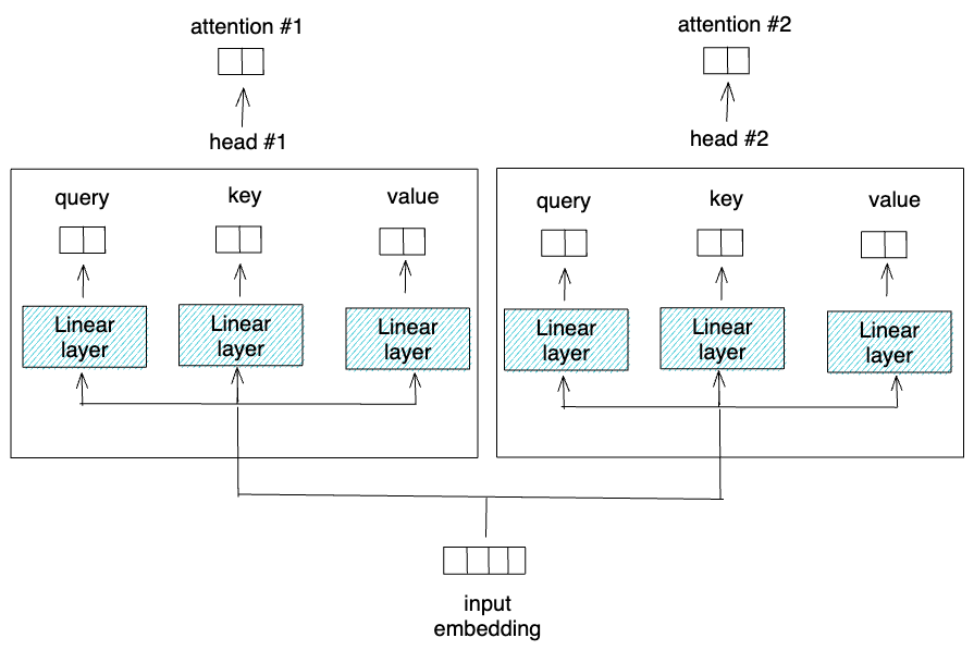
In the end, we need to concatenate the output from each single self-attention layer and then project it into an additional linear layer.

class MultiHeadAttention(nn.Module):
    def __init__(self, h, d_model, dropout=0.1):
        super().__init__()
        assert d_model % h == 0
        d_k = d_model // h
        self.multi_head = nn.ModuleList([SingleHeadAttention(d_model, d_k) for _ in range(h)])
        self.lin_agg = nn.Linear(d_model, d_model)

    def forward(self, x):
        x = torch.cat([head(x) for head in self.multi_head], dim=-1)
        return self.lin_agg(x)
And that's it. The output tensor of this multi-head attention layer has the same dimensionality as the input.
mult_att = MultiHeadAttention(h=2, d_model=4)
output_mult_att = mult_att(output_pe)
print(f'Size of output embedding after multi-head attention: {output_mult_att.size()}')

# Output
'''
Size of output embedding after multi-head attention: torch.Size([1, 3, 4])
'''
Normalization Layer and Residual Connection
If we take a look at the architecture of Transformer encoder block, we need to add the output of multi-head attention with the input of multi-head attention (also called residual connection) and then normalize it.

The reason behind these two operations is so that the Transformer model can converge faster during training process and they can also help the model to perform more accurately.
class LayerNorm(nn.Module):
    def __init__(self, d_model, eps=1e-6):
        super(LayerNorm, self).__init__()
        self.a_2 = nn.Parameter(torch.ones(d_model))
        self.b_2 = nn.Parameter(torch.zeros(d_model))
        self.eps = eps

    def forward(self, x):
        mean = x.mean(-1, keepdim=True)
        std = x.std(-1, keepdim=True)
        return self.a_2 * (x - mean) / (std + self.eps) + self.b_2

class ResidualConnection(nn.Module):
    def __init__(self, d_model, dropout=0.1):
        super().__init__()
        self.norm = LayerNorm(d_model)
        self.dropout = nn.Dropout(dropout)

    def forward(self, x1, x2):
        return self.dropout(self.norm(x1 + x2))
Again, the output tensor dimension after the residual connection and normalization layer would be the same as the output tensor dimension of multi-head attention layer.
res_conn_1 = ResidualConnection(d_model=4)
output_res_conn_1 = res_conn_1(output_pe, output_mult_att)

print(f'Size of output embedding after residual connection: {output_res_conn_1.size()}')

# Output
'''
Size of output embedding after residual connection: torch.Size([1, 3, 4])
'''
Feed Forward Layer
The output of residual connection and normalization layer then become the input of a feed-forward layer. This layer is just an ordinary linear layer, as you can see below:
class FeedForward(nn.Module):
    def __init__(self, d_model, d_ff, dropout=0.1):
        super().__init__()
        self.w_1 = nn.Linear(d_model, d_ff)
        self.w_2 = nn.Linear(d_ff, d_model)
        self.dropout = nn.Dropout(dropout)

    def forward(self, x):
        return self.w_2(self.dropout(self.w_1(x).relu()))
This layer also won't change the dimension of our tensor.
ff = FeedForward(d_model=4, d_ff=12)
output_ff = ff(output_res_conn_1)

print(f'Size of output embedding after feed-forward network: {output_ff.size()}')

# Output
'''
Size of output embedding after feed-forward network: torch.Size([1, 3, 4])
'''
After the feed-forward layer, we need to apply the second residual connection, in which we add the output of feed-forward layer with the input of feed-forward layer. After the addition, we normalize the tensor with normalization layer as described in Normalization Layer section above.
res_conn_2 = ResidualConnection(d_model=4)
output_res_conn_2 = res_conn_2(output_res_conn_1, output_ff)

print(f'Size of output embedding after second residual: {output_res_conn_2.size()}')

# Output
'''
Size of output embedding after second residual: torch.Size([1, 3, 4])
'''
Transformer Encoder Stack
The process from multi-head self-attention layer until the normalization layer after the feed-forward layer above corresponds to one single Transformer encoder stack.

Now we can encapsulate all of the process above in a class called SingleEncoder() below:
class SingleEncoder(nn.Module):
    def __init__(self, d_model, self_attn, feed_forward, dropout):
        super().__init__()
        self.self_attn = self_attn
        self.feed_forward = feed_forward
        self.res_1 = ResidualConnection(d_model, dropout)
        self.res_2 = ResidualConnection(d_model, dropout)

        self.d_model = d_model

    def forward(self, x):
        x_attn = self.self_attn(x)
        x_res_1 = self.res_1(x, x_attn)
        x_ff = self.feed_forward(x_res_1)
        x_res_2 = self.res_2(x_res_1, x_ff)

        return x_res_2
In its application, we usually use several Transformer encoders instead of just one. BERT-base model, for example, uses 12 stacks of Transformer encoders.
class EncoderBlocks(nn.Module):
    def __init__(self, layer, N):
        super().__init__()
        self.layers = nn.ModuleList([layer for _ in range(N)])
        self.norm = LayerNorm(layer.d_model)

    def forward(self, x):
        for layer in self.layers:
            x = layer(x)
        return self.norm(x)
With the EncoderBlocks() above, then we can initialize several stacks of Transformer encoders according to our need.
Model Training
Now that we know the inner architecture of a Transformer encoder, now let's use it to train our data for a text classification purpose.
Model Definition
In this article, we will use six stacks of Transformer encoders. The hidden size would be 300 and there will be four different heads in the multi-head self-attention layer. You can tweak these values according to your own need.
class TransformerEncoderModel(nn.Module):
    def __init__(self, vocab_size, d_model, nhead, d_ff, N,
                dropout=0.1):
        super().__init__()
        assert d_model % nhead == 0, "nheads must divide evenly into d_model"

        self.emb = Embeddings(d_model, vocab_size)
        self.pos_encoder = PositionalEncoding(d_model=d_model, vocab_size=vocab_size)

        attn = MultiHeadAttention(nhead, d_model)
        ff = FeedForward(d_model, d_ff, dropout)
        self.transformer_encoder = EncoderBlocks(SingleEncoder(d_model, attn, ff, dropout), N)
        self.classifier = nn.Linear(d_model, 2)
        self.d_model = d_model

    def forward(self, x):
        x = self.emb(x) * math.sqrt(self.d_model)
        x = self.pos_encoder(x)
        x = self.transformer_encoder(x)
        x = x.mean(dim=1)
        x = self.classifier(x)
        return x

model = TransformerEncoderModel(len(vocab), d_model=300, nhead=4, d_ff=50,
                                    N=6, dropout=0.1).to(device)
If you notice, we also add an additional linear layer on top of the output of the last Transformer encoder stack. This linear layer will act as the classifier. Since we only have two distinct classes (spam/ham), then the output of this linear layer would be two.
Also, one more important thing that we need to address is the fact that the output of the final stack would be [batch, no_of_sequence, hidden_size] , while our final linear layer expects an input of [batch, hidden_size] . There are several methods that we can do to match the output of the stack with the input of linear layer.
BERT, for example, uses only the output of a special token called [CLS] that is prepended into our sequence before the positional encoding steps in the Transformer architecture above. Here, we don't have that special [CLS] token. Thus, what we do instead is averaging all of the output embedding values after the last encoder stack.
Data Loader
Next, we need to create a data loader for our training data such that it will be supplied into our model in batches during the training process.
class TextDataset(torch.utils.data.Dataset):

  def __init__(self, input_data):
      self.text = input_data['Message'].values.tolist()
      self.label = [int(label2id[i]) for i in input_data['Category'].values.tolist()]

  def __len__(self):
      return len(self.label)

  def get_sequence_token(self, idx):
      sequence = [vocab[word] for word in tokenizer(self.text[idx])]
      len_seq = len(sequence)
      return sequence, len_seq

  def get_labels(self, idx):
      return self.label[idx]

  def __getitem__(self, idx):
      sequence, len_seq = self.get_sequence_token(idx)
      label = self.get_labels(idx)
      return sequence, label, len_seq

def collate_fn(batch):

    sequences, labels, lengths = zip(*batch)
    max_len = max(lengths)

    for i in range(len(batch)):
        if len(sequences[i]) != max_len:
          for j in range(len(sequences[i]),max_len):
            sequences[i].append(0)

    return torch.tensor(sequences, dtype=torch.long), torch.tensor(labels, dtype=torch.long)
In addition to the dataloader class, we also need to create supplementary function called collate_fn() above. This function is essential because, in order to supply our training data in batches, each batch needs to have the same dimension.
Since we're dealing with text data with varying sentence length, then the dimension of each batch isn't guaranteed to be the same. In the collate_fn , we first fetch the maximum length of a sequence in a batch, and then add a bunch of tokens to the shorter sequence until its length equals to the length of the longest sequence in the batch.
Another method that you can use is by defining the maximum number of tokens. Next, you can truncate the sentence if it has more tokens than the maximum value or add a bunch of tokens **** if it has fewer tokens than the maximum value.
Training Loop
Now that we have defined the model architecture and the data loader class, then we can start to train the model.
def train(model, dataset, epochs, lr, bs):

    criterion = nn.CrossEntropyLoss()
    optimizer = torch.optim.Adam((p for p in model.parameters()
      if p.requires_grad), lr=lr)
    train_dataset = TextDataset(dataset)
    train_dataloader = DataLoader(train_dataset, num_workers=1, batch_size=bs, collate_fn=collate_fn, shuffle=True)

    # Training loop
    for epoch in range(epochs):
        total_loss_train = 0
        total_acc_train = 0
        for train_sequence, train_label in tqdm(train_dataloader):

            # Model prediction
            predictions = model(train_sequence.to(device))
            labels = train_label.to(device)
            loss = criterion(predictions, labels)

            # Calculate accuracy and loss per batch
            correct = predictions.argmax(axis=1) == labels
            acc = correct.sum().item() / correct.size(0)
            total_acc_train += correct.sum().item()
            total_loss_train += loss.item()

            # Backprop
            loss.backward()
            torch.nn.utils.clip_grad_norm_(model.parameters(), 0.5)
            optimizer.step()

        print(f'Epochs: {epoch + 1} | Loss: {total_loss_train / len(train_dataset): .3f} | Accuracy: {total_acc_train / len(train_dataset): .3f}')

epochs = 15
lr = 1e-4
batch_size = 4
train(model, df_train, epochs, lr, batch_size)
And you'll get the output that looks something like this:

Model Prediction
After we train the model, we can naturally use it to predict unseen data on our test set. To do so, first we need to create a function that encapsulates data preprocessing step and the model prediction step.
def predict(text):
  sequence = torch.tensor([vocab[word] for word in tokenizer(text)], dtype=torch.long).unsqueeze(0)
  output = model(sequence.to(device))
  prediction = id2label[output.argmax(axis=1).item()]

  return prediction
Now if we want to predict a text from our test set, we can just call the function above:
idx = 24
text = df_test['Message'].values.tolist()[idx]
gt = df_test['Category'].values.tolist()[idx]
prediction = predict(text)

print(f'Text: {text}')
print(f'Ground Truth: {gt}')
print(f'Prediction: {prediction}')

# Output
'''
Text: This is the 2nd time we have tried 2 contact u. U have won the £750 Pound prize. 2 claim is easy, call 087187272008 NOW1! Only 10p per minute. BT-national-rate.
Ground Truth: spam
Prediction: spam
'''
idx = 35
text = df_test['Message'].values.tolist()[idx]
gt = df_test['Category'].values.tolist()[idx]
prediction = predict(text)

print(f'Text: {text}')
print(f'Ground Truth: {gt}')
print(f'Prediction: {prediction}')

# Output
'''
Text: Morning only i can ok.
Ground Truth: ham
Prediction: ham
'''
Conclusion
In this article, we have discussed the step-by-step process to utilize the encoder part of Transformer to classify text. As you already know, there are a lot of large language models out there that use the encoder part of Transformer. BERT, as an example, achieved state-of-the-art performance in many language tasks, thanks to its Transformer-encoder architecture combined with a large corpus of training data.
I hope this article helps you to getting started with Transformer architecture. As usual, you can find the code implemented in this article via this notebook.
