The Best Optimization Algorithm for Your Neural Network

Developing any machine learning model involves a rigorous experimental process that follows the idea-experiment-evaluation cycle.

The above cycle is repeated multiple times until satisfactory performance levels are achieved. The "experiment" phase involves both the coding and the training steps of the machine learning model. As models become more complex and are trained over much larger datasets, training time inevitably expands. As a consequence, training a large deep neural network can be painfully slow.
Fortunately for Data Science practitioners, there exist several techniques to accelerate the training process, including:
- Transfer Learning.
- Weight Initialization, as Glorot or He initialization.
- Batch Normalization for training data.
- Picking a reliable activation function.
- Use a faster optimizer.
While all the techniques I pointed out are important, in this post I will focus deeply on the last point. I will describe multiple algorithm for neural network parameters optimization, highlighting both their advantages and limitations.
In the last section of this post, I will present a visualization displaying the comparison between the discussed optimization algorithms.
For practical implementation, all the code used in this article can be accessed in this GitHub repository:
Batch Gradient Descent
Traditonally, Batch Gradient Descent is considered the default choice for the optimizer method in neural networks.
After the neural network generates predictions for the entire training set X, we compare the network's predictions to the actual labels of each training point. This is done to compute a cost function J(W,b), which is a scalar representation of the capacity of the model to yield accurate predictions. The Gradient Descent optimization algorithm uses the cost function as a guide to tune every network's parameter. This iterative process continues until the cost function is close to zero, or it can't be reduced further. What GD does is to adjust each weight and bias of the network in a certain direction. The chosen direction is the one that reduces the cost function the most.
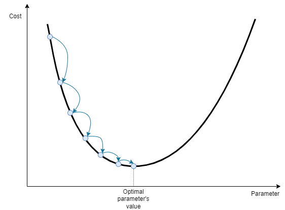
In visual terms, take the image above for reference. Gradient descent starts at the leftmost blue point. By analyzing the gradient of the cost function around the starting point, it adjusts the parameter (x-axis value) to the right. This process is repeated multiple times until the algorithm ends up with a very good approximation of the optimum.
If the cost function has 2 input parameters, the function is not a line but instead, it creates a three-dimensional surface. The batch gradient descent steps can be displayed considering the level curves of the surface:

A neural network consists of thousands or millions of parameters that affect the cost functions. While visualizing million-dimensional representations is infeasible, mathematical equations are useful to understand the gradient descent process.
At first, we compute the cost function J(W,b), which is a function of the network's weights W and biases b. Then, the backpropagation algorithm computes the derivative of the cost function with respect to each weight and bias of each layer of the network:


Knowing the direction towards which to adjust the parameters, we update them. The magnitude of each parameter's update is regulated by the gradient itself and by the learning rate alpha. Alpha is a hyperparameter of the optimization algorithm and its value is typically maintained constant.

Batch Gradient Descent offers several advantages:
- Simplicity: It's a straightforward and easy-to-understand method.
- Hyperparameter Management: It requires tuning only one hyperparameter, the learning rate.
- Optimality: For convex cost functions, it reliably reaches the global optimum with a reasonable learning rate.
The disadvantages of gradient descent are:
- Computational Intensity: It can be slow, particularly for large training sets, as it updates parameters after evaluating all examples.
- Local Optima and Saddle Points: It might get stuck in local optima or saddle points, slowing convergence.
- Gradient Issues: It is prone to vanishing gradient issues.
- Memory Usage: It requires storing the entire training data in CPU/GPU memory.
Mini-Batch Gradient Descent
In batch gradient descent algorithm all training examples are used to calculate a single improvement step. The step will be the most accurate, as it considers all the available information. However, this approach often is impractically slow in real-world applications, suggesting the implementation of faster alternatives.
The most common solution is called Mini-Batch Gradient Descent, and it uses only a small subset of the training data in order to update the weights' values.
Consider the whole training set X, and the associated labels Y:

where m represents the number of training examples.
Rather than feeding the whole batch to the optimization algorithm, we process only a small portion of the training set. Let's say we feed the algorithm the subsets X^t and Y^t, each containing 512 training examples:

For instance, if the total training set contains 5,120,000 points, it can be divided into 10,000 mini-batches, each containing 512 examples.
For each mini-batch, we perform the classical gradient descent operations:
- Compute the cost relative to the mini-batch t, J^t(W,b).
- Perform backpropagation to compute the gradients of J^t(W,b) with respect to each weight and bias.
- Update the parameters.
The green line in the image below shows a typical optimization path of the mini-batch gradient descent. While batch gradient descent follows a more direct path to the optimal point, mini-batch gradient descent appears to take several unnecessary steps, due to its limited dataset at each iteration.

The reason for that is that mini-batch gradient descent, at any time t, has only a small portion of the training set to compute its decision on. With that limitation on the available information, it's clear that the route followed is not the most direct.
However, the significant advantage of mini-batch gradient descent, is that each step is extremely fast to be computed since the algorithm needs to evaluate only a small portion of the data instead of the whole training set. In our example, each step requires the evaluation of only 512 data points instead of 5 million. This is also the reason why almost no real application, requiring a large amount of data, uses batch gradient descent.
As the image shows, with mini-batch gradient descent there is no guarantee that the cost at iteration t+1 is lower than the cost at iteration t, but, if the problem is well defined, the optimization algorithm reaches an area very close to the optimal point really quickly.
The choice of the mini-batch size represents an additional hyperparameter of the network's training process. A batch size equal to the total number of examples (m) corresponds to the batch gradient descent optimization. Instead, if m=1 we are performing Stochastic Gradient Descent, where each training example is a mini-batch.
If the training set is small, batch gradient descent can be a valid option, otherwise, popular mini-batch sizes like 32, 64, 128, 256, and 512 are commonly considered. For some reason, a batch size equal to a power of 2 seems to perform better.
While stochastic gradient descent with a batch size of 1 is an option, it tends to be extremely noisy, and it can bounce further away from the minima. Moreover, stochastic gradient descent is very inefficient if we consider the computation time per example, as it cannot exploit the benefits of vectorization.
Gradient Descent with Momentum
Recall that in both Batch and Mini-Batch Gradient Descent, the parameter update follows a defined formula:

Therefore, in this equation, the size of each optimization step is determined by the learning rate, a fixed quantity, and the gradient, which is computed at a specific point of the cost function.
When the gradient is computed in a nearly flat section of the cost function, it will be very small, leading to a proportionally small step of gradient descent. Consider the difference the gradient difference at points A and B of the image below.

Momentum Gradient Descent overcomes this issue. We can imagine momentum gradient descent as a bowling ball rolling down a hill, which shape is defined by the cost function. If the ball begins its descent from a steep portion of the slope, its movement begins slowly but it will quickly gain velocity and momentum. Due to its momentum, the ball maintains great velocity even through a -flat area of the slope.
This is the core concept of momentum gradient descent: the algorithm will consider previous gradients, and not only the one computed at iteration t. Similar to the bowling ball analogy, the gradient computed at iteration t defines the acceleration and not the speed of the ball.
Both weights and biases' velocities are computed at each step using the previous velocity and the current iteration's gradient:

The parameter beta, known as momentum, regulates how much the new velocity value is determined from the current slope or from the past velocity value.
Finally, parameters are updated using the computed velocity:

Momentum Gradient Descent has proven superior performance compared to Mini-Batch Gradient Descent in most applications. The main drawback of Momentum Gradient Descent, with respect to standard Gradient Descent, is that it requires an additional parameter to tune. However, practice shows how a value of beta equal to 0.9 works effectively.
RMS Prop
Consider a cost function shaped similarly to an elongated bowl, where the minimum point is located in the narrowest part. The function's contour is described by the level curves in the image below.

In cases where the starting point is far away from the minimum, Gradient Descent, also with the momentum variation, starts by following the steepest slope, which, in the picture above, is not the optimal path towards the minimum. The key idea of RMS Prop optimization algorithm is to correct the direction early and to aim for the global minimum more promptly.
Similarly to Momentum Gradient Descent, RMS Prop requires fine-tuning through an additional hyperparameter known as the decay rate. Through practical experience, it has been proven that setting the decay rate to 0.9 is a good choice for most problems.
Adam
Adam and its variations are probably the most employed optimization algorithms for neural networks. Adam, which stands for Adaptive Moment Estimation, is derived from the combinations of Momentum Gradient Descent and RMS Prop together.
As a mix of the two optimization methods, Adam needs two additional hyperparameters to be tuned (besides the learning rate alpha). We call them _beta1 and _beta2 and they are the hyperparameters used respectively in Momentum and in RMS Prop. As happened for the other discussed algorithms, effective default choices for _beta1 and _beta2 exist: _beta1 is usually set to 0.9 and _beta2 to 0.999. In Adam appears also a parameter epsilon that works as a smoothing term and it is nearly always set to a small value like e-7 or e-8.
Adam optimization algorithm outperforms all the above-mentioned methods in most cases. The only exceptions can be very simple problems where simpler methods work faster. The efficiency of Adam does come with a trade-off: the need to fine-tune two additional parameters. However, in my opinion it is a small price to pay for its efficiency.
Nadam and AdaMax
It is worth citing two algorithms born as modifications of the widely used Adam optimization: Nadam and AdaMax.
Nadam, short of Nesterov-accelerated Adaptive Moment Estimation, enhances Adam by incorporating Nesterov Accelerated Gradient (NAG) into its framework. This means that Nadam not only benefits from the adaptive learning rates and momentum of Adam, but also from the NAG component, a technique that helps the algorithm predict the next step more accurately. Especially in high-dimensional spaces, Nadam converges faster and more effectively.
AdaMax, instead, adopts a slightly different approach. While Adam calculates adaptive learning rates based on both the first and second moments of the gradients, AdaMax focuses only on the maximum norm of the gradients. AdaMax's simplicity and efficiency in handling sparse gradients make it an appealing choice for training deep neural networks, especially in tasks involving sparse data.
Optimization Algorithms Comparison
In order to practically test and visualize the performance of each discussed optimization algorithm, I trained a simple deep neural network with each one of the above optimizers. The job of the network is to classify fashion items displayed in 28×28 pixels images. The dataset is called Fashion MNIST (MIT licensed) and is composed of 70,000 small grey-scale images of clothing items.
The algorithm I used to test different optimizers is presented in the following snippet and, more completely in the GitHub repository linked below.
# Load data
(X_train, y_train), (X_test, y_test) = load_my_data()
# Print an example
#print_image(X_train, 42)

# Normalize the inputs
X_train = X_train / 255.
X_test = X_test / 255.

# Define the optimizers to test
my_optimizers = {"Mini-batch GD":tf.keras.optimizers.SGD(learning_rate = 0.001, momentum = 0.0),
                 "Momentum GD":tf.keras.optimizers.SGD(learning_rate = 0.001, momentum = 0.9),
                 "RMS Prop":tf.keras.optimizers.RMSprop(learning_rate = 0.001, rho = 0.9),
                 "Adam":tf.keras.optimizers.Adam(learning_rate = 0.001, beta_1 = 0.9, beta_2 = 0.999)
    }

histories = {}
for optimizer_name, optimizer in my_optimizers.items():
    # Define a neural network

    my_network = tf.keras.models.Sequential([
                tf.keras.layers.Flatten(input_shape=(28, 28)),
                tf.keras.layers.Dense(128, activation='relu'),
                tf.keras.layers.Dense(64, activation='relu'),
                tf.keras.layers.Dense(10, activation='softmax')
                ])
    # Compile the model
    my_network.compile(optimizer=optimizer,
                       loss='sparse_categorical_crossentropy', # since labels are more than 2 and not one-hot-encoded
                       metrics=['accuracy'])

    # Train the model
    print('Training the model with optimizer {}'.format(optimizer_name))
    histories[optimizer_name] = my_network.fit(X_train, y_train, epochs=50, validation_split=0.1, verbose=1)

# Plot learning curves
for optimizer_name, history in histories.items():
    loss = history.history['loss']
    epochs = range(1,len(loss)+1)
    plt.plot(epochs, loss, label=optimizer_name)
    plt.legend(loc="upper right")
    plt.xlabel("Epoch")
plt.ylabel("Loss")The resulting plot is visualized in this line chart:

We can immediately see how the Momentum Gradient Descent (yellow line) is considerably faster than the standard Gradient Descent (blue line). Instead, RMS Prop (green line) seems to obtain similar results as Momentum Gradient Descent. This may be due to several reasons such as not perfectly tuned hyperparameters or a too-simple neural network. Finally, Adam optimizer (red line) looks superior, by a margin, to all the other methods.
Learning Rate Decay
I want to include learning rate decay in this post because, even though it is not strictly an optimization algorithm, it is a powerful technique to accelerate the network's learning process.

Learning rate decay consists of the reduction of the learning rate hyperparameter alpha over the epochs. Theis adjustment is essential because at the initial stages of the optimization, the algorithm can afford to take bigger steps but, as it approaches the minimum point, we prefer to make smaller steps so that it will bounce in an area closer to the minimum.
There exist several methods to decrease the learning rate over iterations. One approach is described by the following formula:

where the decay rate is an additional parameter to tune.
Alternatively, other possibilities are:


The first one is called Exponential Learning Rate Decay, and in the second one, parameter k is a constant.
Finally, it is also possible to apply a discrete learning rate decay, such as halving it after every t iterations, or decreasing it manually.

Conclusion
Time is a valuable, but also limited, resource for every data science practitioner. For this reason, mastering the tools to speed up a learning algorithm training can make a difference.
In this article, we have seen how the standard Gradient Descent optimizer is an outdated tool, and there exist several alternatives that provide better solutions in less time.
Choosing the right optimizer for a given Machine Learning application is not always easy. It depends on the task and there is not a clear consensus yet on which one is the best. However, as we saw above, Adam optimizer with the proposed hyperparameters' values is a valid choice most of the time, and knowing the functioning principle of the most popular ones is an excellent starting point.
If you liked this story, consider following me to be notified of my upcoming projects and articles!
Here are some of my past projects:
Social Network Analysis with NetworkX: A Gentle Introduction
Use Deep Learning to Generate Fantasy Names: Build a Language Model from Scratch
Support Vector Machine with Scikit-Learn: A Friendly Introduction
References
- Gradient descent – Wikipedia.org
- Dive into Deep Learning – Aston Zhang, Zachary C. Lipton, Mu Li, and Alexander J. Smola
- Delving Deep into Rectifiers: Surpassing Human-Level Performance on ImageNet Classification – Kaiming He, Xiangyu Zhang, Shaoqing Ren, Jian Sun
- Improving Deep Neural Networks: Hyperparameter Tuning, Regularization and Optimization – Andrew Ng
- Understanding the difficulty of training deep feedforward neural networks – Xavier Glorot, Yoshua Bengio
- Hands-On Machine Learning with Scikit-Learn, Keras, and TensorFlow, 2nd Edition – Aurélien Géron
- Keras Python library
