Two Advanced SQL Techniques That Can Drastically Improve Your Queries

Sql is the bread and butter of every data professional. It doesn't matter if you are a data analyst, data scientist, or data engineer, you need to have a solid understanding of how to write clean and efficient SQL queries.
This is because behind any rigorous data analysis or any sophisticated machine learning model is the underlying data itself, and this data has to come from somewhere.
Hopefully after reading my introductory blog post to SQL, you would have already learned that SQL stands for Structured Query Language and it is a language that is used to retrieve data from a relational database.
In that blog post, we went over some fundamental SQL commands such as SELECT, FROM, and WHERE which should cover most of the basic queries you will come across when using SQL.
But what happens if those simple commands are simply not enough? What happens if the data you want demands a more robust approach to query?
Well, look no further because today, we will go over two new SQL techniques that you can add to your toolkit that will take your queries to the next level. These techniques are called Common Table Expression (CTE) and Window Functions.
To help us learn these techniques, we will be using an online SQL editor called DB Fiddle (set to SQLite v3.39) and the taxi trip duration dataset sourced from Google Cloud (NYC Open Data license).
Data Preparation
If you are not interested to learn how I prepared the dataset, feel free to skip past this section and paste the following code onto DB fiddle to generate the schema.
CREATE TABLE taxi (
  id varchar,
  vendor_id integer,
  pickup_datetime datetime,
  dropoff_datetime datetime,
  trip_seconds integer,
  distance float
);

INSERT INTO taxi
VALUES
('id2875421', 2, '2016-03-14 17:24:55', '2016-03-14 17:32:30', 455, 0.93),
('id2377394', 1, '2016-06-12 00:43:35', '2016-06-12 00:54:38', 663, 1.12),
('id3858529', 2, '2016-01-19 11:35:24', '2016-01-19 12:10:48', 2124, 3.97),
('id3504673', 2, '2016-04-06 19:32:31', '2016-04-06 19:39:40', 429, 0.92),
('id2181028', 2, '2016-03-26 13:30:55', '2016-03-26 13:38:10', 435, 0.74),
('id0801584', 2, '2016-01-30 22:01:40', '2016-01-30 22:09:03', 443, 0.68),
('id1813257', 1, '2016-06-17 22:34:59', '2016-06-17 22:40:40', 341, 0.82),
('id1324603', 2, '2016-05-21 07:54:58', '2016-05-21 08:20:49', 1551, 3.55),
('id1301050', 1, '2016-05-27 23:12:23', '2016-05-27 23:16:38', 255, 0.82),
('id0012891', 2, '2016-03-10 21:45:01', '2016-03-10 22:05:26', 1225, 3.19),
('id1436371', 2, '2016-05-10 22:08:41', '2016-05-10 22:29:55', 1274, 2.37),
('id1299289', 2, '2016-05-15 11:16:11', '2016-05-15 11:34:59', 1128, 2.35),
('id1187965', 2, '2016-02-19 09:52:46', '2016-02-19 10:11:20', 1114, 1.16),
('id0799785', 2, '2016-06-01 20:58:29', '2016-06-01 21:02:49', 260, 0.62),
('id2900608', 2, '2016-05-27 00:43:36', '2016-05-27 01:07:10', 1414, 3.97),
('id3319787', 1, '2016-05-16 15:29:02', '2016-05-16 15:32:33', 211, 0.41),
('id3379579', 2, '2016-04-11 17:29:50', '2016-04-11 18:08:26', 2316, 2.13),
('id1154431', 1, '2016-04-14 08:48:26', '2016-04-14 09:00:37', 731, 1.58),
('id3552682', 1, '2016-06-27 09:55:13', '2016-06-27 10:17:10', 1317, 2.86),
('id3390316', 2, '2016-06-05 13:47:23', '2016-06-05 13:51:34', 251, 0.81),
('id2070428', 1, '2016-02-28 02:23:02', '2016-02-28 02:31:08', 486, 1.56),
('id0809232', 2, '2016-04-01 12:12:25', '2016-04-01 12:23:17', 652, 1.07),
('id2352683', 1, '2016-04-09 03:34:27', '2016-04-09 03:41:30', 423, 1.29),
('id1603037', 1, '2016-06-25 10:36:26', '2016-06-25 10:55:49', 1163, 3.03),
('id3321406', 2, '2016-06-03 08:15:05', '2016-06-03 08:56:30', 2485, 12.82),
('id0129640', 2, '2016-02-14 13:27:56', '2016-02-14 13:49:19', 1283, 2.84),
('id3587298', 1, '2016-02-27 21:56:01', '2016-02-27 22:14:51', 1130, 3.77),
('id2104175', 1, '2016-06-20 23:07:16', '2016-06-20 23:18:50', 694, 2.33),
('id3973319', 2, '2016-06-13 21:57:27', '2016-06-13 22:12:19', 892, 1.57),
('id1410897', 1, '2016-03-23 14:10:39', '2016-03-23 14:49:30', 2331, 6.18);
After running SELECT * from taxi, you should get a resulting table that looks like this.

For the keen beans who are wondering how this table actually came about, I filtered the data to the first 30 rows and only kept the columns that you see above. As for the distance field, I computed the orthodromic distance between the pick-up and drop-off coordinates (latitude and longitude).
The orthodromic distance is the shortest distance between two points on a sphere, so this actually turns out to be an underestimate of the real distance travelled by the taxi. However, for the purpose of what we are doing today, we can ignore this for now.
The formula to calculate the orthodromic distance can be found here. Now, back to SQL.
Common Table Expression (CTE)
A common table expression (CTE) is a temporary table that you return within a query. You can think of it as a query within a query. They help to not only split your queries into more readable chunks but you can write new queries based on a CTE that has been defined.
To demonstrate this, suppose we want to analyze taxi trips split by the hour of the day and filter to trips that took place between the months of January and March 2016.
SELECT CAST(STRFTIME('%H', pickup_datetime) AS INT) AS hour_of_day,
       trip_seconds,
       distance
FROM taxi
WHERE pickup_datetime > '2016-01-01'
  AND pickup_datetime < '2016-04-01'
ORDER BY hour_of_day;
Straightforward enough; let's take this one step further.
Suppose now we want to compute the number of trips and the average speed for each of these hours. This is where we can utilize a CTE to first obtain a temporary table like the one we observe above, followed by a subsequent query to count the number of trips and compute the average speed group by hour of the day.
The way you would define a CTE is by using the WITH and AS statements.
WITH relevantrides AS
(
SELECT CAST(STRFTIME('%H', pickup_datetime) AS INT) AS hour_of_day,
       trip_seconds,
       distance
FROM taxi
WHERE pickup_datetime > '2016-01-01'
  AND pickup_datetime < '2016-04-01'
ORDER BY hour_of_day
)
SELECT hour_of_day,
       COUNT(1) AS num_trips,
       ROUND(3600 * SUM(distance) / SUM(trip_seconds), 2) AS avg_speed
FROM relevantrides
GROUP BY hour_of_day
ORDER BY hour_of_day;
An alternative to using a CTE is simply wrapping the temporary table within a FROM statement (see code below), which would give you the same result. However, this is not advisable from a code readability standpoint. Moreover, imagine if we wanted to create more than just one temporary table.
SELECT hour_of_day,
       COUNT(1) AS num_trips,
       ROUND(3600 * SUM(distance) / SUM(trip_seconds), 2) AS avg_speed
FROM (
 SELECT CAST(STRFTIME('%H', pickup_datetime) AS INT) AS hour_of_day,
           trip_seconds,
           distance
 FROM taxi
 WHERE pickup_datetime > '2016-01-01'
    AND pickup_datetime < '2016-04-01'
 ORDER BY hour_of_day
)
GROUP BY hour_of_day
ORDER BY hour_of_day;
Bonus: an interesting insight we can pull from this exercise is that taxis tend to move slower (lower average speed) during peak hours most likely due to heavier traffic as people travel to and back from work.
Window Functions
Window functions perform aggregate operations on groups of rows but they produce a result for each row in the original table.
To fully understand how window functions work, it is helpful to first do a quick recap of aggregation via GROUP BY.
Let's say we wish to compute a list of summary statistics by month using the taxi dataset.
SELECT CAST(STRFTIME('%m', pickup_datetime) AS INT) AS month,
       COUNT(1) AS trip_count,
       ROUND(SUM(distance), 3) AS total_distance,
       ROUND(AVG(distance), 3) AS avg_distance,
       MIN(distance) AS min_distance,
       MAX(distance) AS max_distance
FROM taxi
GROUP BY month;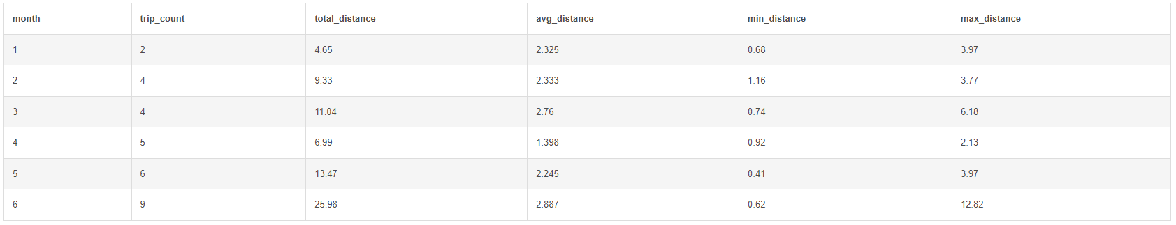
In the example above, we have computed the count, sum, average, minimum, and maximum distance travelled for each individual month in the dataset. Notice how our original taxi table with 30 rows has now been collapsed into six rows, one for each individual month.
So, what is actually happening behind the scenes? Firstly, SQL grouped all 30 rows in the original table based on their months. It then applied the relevant calculations based on the values in these individual groups.
Let's take January as an example. There are two trips in the dataset that took place in the month of January, with distance travelled of 3.97 and 0.68 respectively. SQL then calculated the count, sum, average, minimum, and maximum based on these two values. The process then repeats for the other months until eventually we get an output that looks like the one above.
Now, hold this thought as we begin to explore how window functions work. There are three broad categories of window functions: aggregate functions, ranking functions, and navigation functions. We will look at examples of each one of them.
Aggregate functions
We have already seen aggregate functions at play in our previous example. Aggregate functions include functions like count, sum, average, minimum, and, maximum.
But where window functions differ from GROUP BY is the number of rows in the final output. Specifically, we saw that after aggregating by months, our output table is left with only six rows (one row for each distinct month).
Window functions, on the other hand, will not summarise the table by the aggregate field, but simply output the result in a new column for each row. The number of rows in the output table will not change. In other words, the output table will always have the same number of rows as the original table.
The syntax to perform a window function is OVER(PARTITION BY ...). You can think of this as the GROUP BY statement in our previous example.
Let's see how this works in practice.
WITH aggregate AS
(
SELECT id,
       pickup_datetime,
       CAST(STRFTIME('%m', pickup_datetime) AS INT) AS month,
       distance
FROM taxi
)
SELECT *,
       COUNT(1) OVER(PARTITION BY month) AS trip_count,
       ROUND(SUM(distance) OVER(PARTITION BY month), 3) AS total_month_distance,
       ROUND(AVG(distance) OVER(PARTITION BY month), 3) AS avg_month_distance,
       MIN(distance) OVER(PARTITION BY month) AS min_month_distance,
       MAX(distance) OVER(PARTITION BY month) AS max_month_distance
FROM aggregate;
Here, we want the same output as last time, but rather than collapsing the table, we want the output displayed as individual rows in a new column.
You would notice the values after the aggregation did not change but rather, they are simply displayed as repeated rows in the table. For example, the first two rows (January) have the same values for trip count, total month distance, average month distance, minimum month distance, and maximum month distance as before. The same applies to the other months.
In case you are wondering how window functions are useful, it helps us compare each row value with the aggregated value. In this instance, we can easily compare the distance travelled in each row with the monthly average, minimum and maximum, and so on.
Ranking functions
Another type of window function is the ranking function. As the name suggests, this ranks a group of rows based on an aggregate field.
WITH ranking AS
(
SELECT id,
       pickup_datetime,
       CAST(STRFTIME('%m', pickup_datetime) AS INT) AS month,
       distance
FROM taxi
)
SELECT *,
       RANK() OVER(ORDER BY distance DESC) AS overall_rank,
       RANK() OVER(PARTITION BY month ORDER BY distance DESC) AS month_rank
FROM ranking
ORDER BY pickup_datetime;
In the example above, we have two ranking columns: one for the overall rank (from 1–30) and one for the monthly rank, both in descending order.
To specify the order when ranking, you will need to use ORDER BY within the OVER statement.
The way you would interpret the results for the first row is that it has the third-longest distance travelled in the whole dataset and the longest distance travelled for the month of January.
Navigation functions
Last but not least, we have navigation functions.
A navigation function assigns a value based on the value in a different row than the current row. Some common navigation functions include FIRST_VALUE, LAST_VALUE, LEAD, and LAG.
SELECT id,
       pickup_datetime,
       distance,
       LAG(distance) OVER(ORDER BY pickup_datetime) AS prev_distance,
       LEAD(distance) OVER(ORDER BY pickup_datetime) AS next_distance
FROM taxi
ORDER BY pickup_datetime;

In the example above, we used the LAG function to return the value of the preceding row and the LEAD function to return the value of the subsequent row. Notice how the first row of the lag column is null whereas the last row of the lead column is null.
SELECT id,
       pickup_datetime,
       distance,
       LAG(distance, 2) OVER(ORDER BY pickup_datetime) AS prev_distance,
       LEAD(distance, 2) OVER(ORDER BY pickup_datetime) AS next_distance
FROM taxi
ORDER BY pickup_datetime;

On a similar note, we can also offset the LEAD and LAG functions, i.e. to start from a particular index or position. When the offset is set to two, you can see that the first two rows of the lag column are null and the last two rows of the lead column are null.
I hope this blog post has helped introduce you to the concepts of Common Table Expression (CTE) and Window Functions.
To summarise, a CTE is a temporary table or a query within a query. They are used to split queries into more readable chunks and you can write new queries against a CTE that has been defined. Window functions, on the other hand, perform aggregation on groups of rows and return the results for each row in the original table.
If you wish to improve on these techniques, I highly encourage you to start implementing them in your SQL queries either at work, solving interview problems, or just playing around with random datasets. Practice makes perfect, am I right?
Support me and other amazing writers by signing up for a Medium membership using the link below. Happy learning!
Don't know what to read next? Here are some suggestions.
10 Most Important SQL Commands Every Data Analyst Needs to Know
Regular Expressions Clearly Explained with Examples
Common Issues that Will Make or Break Your Data Science Project
