A Brief Introduction to Neural Networks : a Classification Problem

Author:Murphy | View: 29652 | Time: 2025-03-23 20:02:18

In a previous tutorial, I covered the basics of neural networks and provided a simple example of using them for a regression problem. I briefly outlined the general process for working with neural networks. In this tutorial, we will delve deeper and learn how to use neural networks for classification tasks. We will follow the same general pipeline as before. However, if you need more background information on neural networks, I recommend reviewing the previous tutorial where I also briefly discussed the concepts of neurons and multi-layer networks.

Not a Medium member? No worries! Continue reading with this friend link.

Table of contents

· 1. Introduction · 2. Problem understanding · 3. Data preparation and preprocessing ∘ 3.1. Data description ∘ 3.2. Data Transformation · 4. Model conception ∘ 4.1. A single unit output ∘ 4.2. One-hot output ∘ 4.3. Convolutional neural networks · 5. Training ∘ 5.1. A single unit output ∘ 5.2. One-hot output ∘ 5.3. Convolution units · 6. Validation ∘ 6.1 Making predictions ∘ 6.2. Learning curves ∘ 6.3. Evaluation on test set ∘ 6.4. Evaluation metrics ∘ 6.5. Display some data · 7. Conclusion

1. Introduction

As previously discussed, the aim of a machine learning solution is to develop a model that can produce the desired output by analyzing a dataset created for a specific task. To achieve this, a series of steps must be followed, which include:

Problem understanding.
Data preparation and pre-processing.
Model conception.
Training the model.
Model evaluation and validation

2. Problem understanding

Before discussing the classification problem that we will solve in this tutorial, it is important to understand that there are several types of classification. Specifically:

Binary classification, when the number of classes is two, such as classifying an email as spam or not.
Multi-class classification, when there are more than two different classes, such as in the Iris dataset where the classes are different types of flowers.
Multi-label classification, when the input has multiple classes, such as classifying images with multiple objects in them.
Furthermore, if the input are images, the classification can be pixel-wise classification (or image segmentation) when each pixel has its own class.

Knowing the type of classification helps us to select the appropriate type of models and the appropriate training parameters such as the loss function. For example, for binary classification the binary_crossentropy function is often used as the loss function whereas categorical_crossentropy is used for multi-class classification.

The problem that we will be solving in this tutorial is handwritten digits classification (multi-class classification). In other words, giving a handwriting digit as an input (from 0 to 9), the model have to identify it and gives what digit is written as an output. We will be testing three types of models: a basic straight forward neural network, a basic straight forward neural network with its output one-hot encoded and a convolutional neural network (CNN).

Let's start be importing the required libraries:

from tensorflow.python.Keras import Input
from tensorflow.python.keras.models import Sequential
from tensorflow.python.keras.layers import Dense, Dropout, Conv2D, MaxPooling2D, Flatten
import tensorflow as tf
import matplotlib.pyplot as plt
import numpy as np
from sklearn.metrics import accuracy_score, precision_score, recall_score, ConfusionMatrixDisplay, f1_score
from sklearn.model_selection import train_test_split
import os

and set the seed so we can regenerate the results:

from numpy.random import seed
seed(1)

from tensorflow import random, config
random.set_seed(1)
config.experimental.enable_op_determinism()

import random
random.seed(2)

3. Data preparation and preprocessing

In order to train our models, we will be using the MNIST dataset which includes a training set of 60,000 examples, and a test set of 10,000 examples. If you wish to use the original dataset in its IDX format, you can check my tutorial for an easy way to explore it. Or, you can simply use the one provided by Keras as follows:

# read dataset:
(x_train, y_train), (x_test, y_test) = tf.keras.datasets.mnist.load_data()

3.1. Data description

We start by displaying the data shape:

print(f"The training data shape: {x_train.shape}, its label shape: {y_train.shape}")
print(f"The test data shape: {x_test.shape}, its label shape: {y_test.shape}")

The training data shape: (60000, 28, 28), its label shape: (60000,)
The test data shape: (10000, 28, 28), its label shape: (10000,)

A single sample is a single channel image (a grayscale image) with a shape of 28×28 pixels. It's important to also display the range of pixel values in the image to determine if data scaling is necessary later on.

print("Minimum value:", np.min(x_train[0]))
print("Maximum value:", np.max(x_train[0]))

Minimum value: 0
Maximum value: 255

Indeed the data scaling is needed later.

Another important factor to display is number of samples in each class. This is important to determine if you are facing imbalanced data:

# Display bars:
fig, axs = plt.subplots(1, 2)
unique, counts = np.unique(y_train, return_counts=True)
axs[0].bar(unique, counts, width=0.4)
axs[0].set_title('Train set')
unique, counts = np.unique(y_test, return_counts=True)
axs[1].bar(unique, counts, width=0.4)
axs[1].set_title('Test set')
plt.show()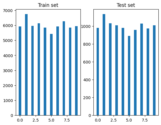

Imbalanced data is a problem in Machine Learning where there is a significant difference in the number of samples between the different classes. In our case, the number of samples is more or less the same.

3.2. Data Transformation

Data transformation is one of the data preprocessing techniques. It includes: data normalization, data encoding, data imputation that fills the missing values, data discretization that transforms continuous features to categorical ones, and dimensionality reduction that reduces the number of features in the dataset. For this example, we will only apply data normalization and data encoding since there is no missing values and there is no need for data discretization and dimensionality reduction.

Data normalization : is a technique used to transform the values of a dataset features so that they are in a specific range. This is usually done to make sure that the data is in a range that is suitable for Neural Networks or other machine learning methods. We normalize the pixels to the range of [0,1]:

Python"># Scale images to the [0, 1] range:
x_train = x_train.astype("float32") / 255
x_test = x_test.astype("float32") / 255

Reshaping (from 2D image to row image): image reshaping or flattening is a common data transformation technique that converts the spatial information into a single row of pixels. It is a necessary step before it can be input into some machine learning models such as multi-layer perceptron (MLP) or linear regression.

We reshape the images for the first two models:

# Data reshaping : from 2D image to row image
x_train = x_train.reshape((x_train.shape[0], x_train.shape[1] * x_train.shape[2]))
x_test = x_test.reshape((x_test.shape[0], x_test.shape[1] * x_test.shape[2]))

Data encoding: one-hot encoding is a technique used to represent categorical variables with a finite number of categories as binary vectors. For a set of n labels, each label is represented by a vector of length n, where each element is 0, except for the element corresponding to the label, which is equal to 1. In our case, the variable we want to predict is the digit class from 0 to 9, which is a finite number of categories that can be represented using one-hot encoding. For example:

The one-hot encoding will be used for the output of the second and third model:

# One-hot encoding:
y_train = tf.keras.utils.to_categorical(y_train, num_classes=10)
y_test = tf.keras.utils.to_categorical(y_test, num_classes=10)

Reshaping (to expand dimension). Reshaping to expand the dimension is usually used in CNNs to increase the number of channels in the input image:

x_train = np.expand_dims(x_train, -1)
x_test = np.expand_dims(x_test, -1)
print(f"The training data shape: {x_train.shape}, its label shape: {y_train.shape}")
print(f"The test data shape: {x_test.shape}, its label shape: {y_test.shape}")

The training data shape: (60000, 28, 28, 1), its label shape: (60000, 10)
The test data shape: (10000, 28, 28, 1), its label shape: (10000, 10)

Let's summarize the data processing: data scaling is applied on the input for all the models, reshaping the input from 2D images to flattened images (row representation) is applied for the first and the second models since they are not CNN based, one-hot encoding is applied on the output of the second and the last model and finally, the input is expanded only for the CNN-based model so the input image becomes a single channel input of size 28×28 pixels.

At the end of the preprocessing stage, the training set is divided into a training and validation set:

# Split dataset:
x_train, x_val, y_train, y_val = train_test_split(x_train, y_train, test_size=0.3, random_state=42)

Our data is reading for training but before that, we need to build our models.

4. Model conception

Now, we will demonstrate the implementation of three different models, starting with a simple fully connected layers model, then gradually improving it. In this tutorial, we will focus on covering the basics that were not covered in the previous tutorial such as the artificial neuron model, activation functions, layers, and multi-layer models.

4.1. A single unit output

The first model is a sequence of fully connected layers, followed by a single unit output. This model is similar to the one used in the previous tutorial. It is easy to implement and can produce good results for this particular example.

Now that we have outlined the general architecture of the model, we need to consider how it will predict the input class (label) based on the available activation functions discussed in the previous tutorial. These functions all return real numbers, but we can use them and round the predicted number to an integer. However, we need to ensure that the output range of the activation function in the final layer includes all possible class values. Therefore, functions such as sigmoid, tanh, and softsign cannot be used in this case.

Fully connected neural network with a single output to predict the input label

Let's create our model! It will have 5 hidden layers, each with 224 units and using the sigmoid activation function. The output layer will have a single unit and will use the relu activation function.

# Create model:
model = Sequential()
model.add(Input(shape=(train_x.shape[1],)))
model.add(Dense(224, activation='sigmoid'))
model.add(Dense(224, activation='sigmoid'))
model.add(Dense(224, activation='sigmoid'))
model.add(Dense(224, activation='sigmoid'))
model.add(Dense(224, activation='sigmoid'))
model.add(Dense(1, activation='relu'))
print(model.summary())

The model summary:

Model: "sequential"
_________________________________________________________________
Layer (type)                 Output Shape              Param #   
=================================================================
dense (Dense)                (None, 224)               175840    
_________________________________________________________________
dense_1 (Dense)              (None, 224)               50400     
_________________________________________________________________
dense_2 (Dense)              (None, 224)               50400     
_________________________________________________________________
dense_3 (Dense)              (None, 224)               50400     
_________________________________________________________________
dense_4 (Dense)              (None, 224)               50400     
_________________________________________________________________
dense_5 (Dense)              (None, 1)                 225       
=================================================================
Total params: 377,665
Trainable params: 377,665
Non-trainable params: 0
_________________________________________________________________

4.2. One-hot output

While the previous model produces good results, as we will see later, better results can be obtained with a smaller model. The key difference is that the output layer is encoded using one-hot representation. Typically, in machine learning, one-hot encoding is implemented using a dense layer of n units (where n is the number of possible categories) and a softmax activation function.

Hmm, I'm not sure that softmax was defined in the previous tutorial, so what is softmax?

"Softmax function converts a vector of values to a probability distribution. The elements of the output vector are in range (0, 1) and sum to 1. Softmax is often used as the activation for the last layer of a classification network because the result could be interpreted as a probability distribution." [1]

The overall model has the following architecture:

Fully connected neural network with a categorical output

To create our model, we will first define the dropout layer which is a regularization technique to prevent overfitting (which will be explained later):

"The Dropout layer randomly sets input units to 0 with a frequency of rate at each step during training time, which helps prevent overfitting. Note that the Dropout layer only applies when training is set to True such that no values are dropped during inference." [2]

In Keras, the dropout layer is defined as following, where rate is a float between 0 and 1 that represents the fraction of the input units to drop :

keras.layers.Dropout(rate, **kwargs)

Now, let's create our model! It will have 2 hidden layers, each with 224 units and using the relu activation function. A dense output layer with 10 units and the softmax activation function will be added. A dropout layer is added after each dense hidden layer to prevent overfitting.

# Create model:
model = Sequential()
model.add(Input(shape=(train_x.shape[1],)))
model.add(Dense(224, activation='relu'))
model.add(Dropout(rate=0.4))
model.add(Dense(224, activation='relu'))
model.add(Dropout(rate=0.4))
model.add(Dense(10, activation='softmax'))
print(model.summary())

The model summary:

Model: "sequential"
_________________________________________________________________
Layer (type)                 Output Shape              Param #   
=================================================================
dense (Dense)                (None, 224)               175840    
_________________________________________________________________
dropout (Dropout)            (None, 224)               0         
_________________________________________________________________
dense_1 (Dense)              (None, 224)               50400     
_________________________________________________________________
dropout_1 (Dropout)          (None, 224)               0         
_________________________________________________________________
dense_2 (Dense)              (None, 10)                2250      
=================================================================
Total params: 228,490
Trainable params: 228,490
Non-trainable params: 0
_________________________________________________________________

As you can see, this model has a smaller number of parameters compared to the previous one (377 665 parameters) and you will see that it will provide better results.

4.3. Convolutional neural networks

So far, we have treated the image as a vector. However, if we want to take advantage of the fact that the image is a 2D matrix, how should we proceed? One approach is to use specialized 2D units. In this section, I will briefly introduce them. However, if you want to learn more about them, I suggest you refer to this tutorial.

Conv2D : applies convolutions using kernels on the input to produce the output (called filters). During training these kernels are updated (trained). Indeed, they play the role of weights in dense layers. In Keras, it is defined as:

keras.layers.Conv2D(
    filters,
    kernel_size,
    **kwargs
)

where: filters is the number of kernels and since each convolution kernel produces an output it also represents the dimensionality of the output space. The kernel_size is the size of kernels that is usually an odd number.

MaxPooling2D : takes the maximum value over an input window. In Keras, it is defined as following, where pool_size is the window size over which to take the maximum:

keras.layers.MaxPooling2D(
    pool_size=(2, 2), **kwargs
)

Now, let's create our CNN model:

# Create model:
model = Sequential()
model.add(Input(shape=(28, 28, 1)))
model.add(Conv2D(32, kernel_size=3, activation="relu"))
model.add(MaxPooling2D(pool_size=2))
model.add(Conv2D(64, kernel_size=3, activation="relu"))
model.add(MaxPooling2D(pool_size=2))
model.add(Flatten())
model.add(Dropout(0.5))
model.add(Dense(n_labels, activation="softmax"))
print(model.summary())

The model summary:

_________________________________________________________________
Layer (type)                 Output Shape              Param #   
=================================================================
conv2d (Conv2D)              (None, 26, 26, 32)        320       
_________________________________________________________________
max_pooling2d (MaxPooling2D) (None, 13, 13, 32)        0         
_________________________________________________________________
conv2d_1 (Conv2D)            (None, 11, 11, 64)        18496     
_________________________________________________________________
max_pooling2d_1 (MaxPooling2 (None, 5, 5, 64)          0         
_________________________________________________________________
flatten (Flatten)            (None, 1600)              0         
_________________________________________________________________
dropout (Dropout)            (None, 1600)              0         
_________________________________________________________________
dense (Dense)                (None, 10)                16010     
=================================================================
Total params: 34,826
Trainable params: 34,826
Non-trainable params: 0
_________________________________________________________________

This model is the smallest one, with only 34,826 parameters which is about 7 times smaller than the previous one. Additionally, you will see that it also achieves the highest performance.

5. Training

As explained in the previous tutorial, training neural networks is updating the weights so the models can fit well on the data. Before starting training, a set of parameters needs to be defined including: the optimizer, the loss function, the batch size, the number of epochs and other metrics to track during training. The choice of loss function and additional metrics heavily depends on the type of output, whether it is a regression or classification problem, etc.

For all the following training, we will set the optimizer to 'adam' which is a good choice if we don't want to handle the learning rate ourselves and the batch size to 128 .

5.1. A single unit output

As this model has a single output layer, the metrics and the loss function that we presented and used in the previous tutorial can be used here. We will set the loss function to mae , the additional metric to mse and the number of epochs to 200:

# Train:
loss = 'mae'
metric = 'mse'
epochs = 200
model.compile(loss=loss, optimizer='adam', metrics=[metric])
history = model.fit(x_train, y_train, epochs=epochs, batch_size=128, verbose=1, validation_data=(x_val, y_val))

By observing the verbose display, we can conclude that the model has learned well and has also been able to generalize (good results for both the train and validation sets):

Epoch 200/200
329/329 [==============================] - 1s 2ms/step - loss: 0.0188 - mse: 0.0525 - val_loss: 0.0946 - val_mse: 0.3838

However, we can achieve better results by using fewer epochs with the one-hot encoding (the second model).

5.2. One-hot output

Unlike the previous model, we use 'categorical_crossentropy' as the loss function and the accuracy as the additional metric. The 'categorical_crossentropy' is a probabilistic loss function that computes the crossentropy loss between the labels and predictions used when there are two or more label classes. It expects labels to be provided in a one_hot representation. As for the accuracy , it is a metric that is more appropriate for classification problems.

# Train:
loss = 'categorical_crossentropy'
metric = 'accuracy'
epochs = 20
model.compile(loss=loss, optimizer='adam', metrics=[metric])
history = model.fit(x_train, y_train, epochs=epochs, batch_size=128, verbose=1, validation_data=(x_val, y_val))

By observing the verbose display, we can conclude that the model has learned well and has also been able to generalize (good results for both the train and validation sets) in only 20 epochs:

Epoch 20/20
329/329 [==============================] - 1s 2ms/step - loss: 0.0469 - accuracy: 0.9838 - val_loss: 0.0868 - val_accuracy: 0.9769

5.3. Convolution units

Now let's train our last model! We use the same loss function and metric as the previous model but with a smaller number of epochs:

# Train:
loss = 'categorical_crossentropy'
metric = 'accuracy'
epochs = 15
model.compile(loss=loss, optimizer='adam', metrics=[metric])
history = model.fit(x_train, y_train, epochs=epochs, batch_size=128, verbose=1, validation_data=(x_val, y_val))

By observing the verbose display, we can say that the model learned well and managed to generalize (good result for the train and validation set) better in only 15 epochs:

Epoch 15/15
329/329 [==============================] - 4s 14ms/step - loss: 0.0340 - accuracy: 0.9892 - val_loss: 0.0371 - val_accuracy: 0.9893

6. Validation

The displayed metrics of the last epochs isn't enough to conclude whether the model has learnt from data or not. The first thing to observe is the learning curves. Then, we can evaluate our model using other metrics. We also test it on a test set if it's available.

But before that, let's see how we can make predictions and get the predicted class.

6.1 Making predictions

Once the model trained, we can start making prediction: predict the class of the image(s) input. In this section, we will see how to get the predicted class for both types of output.

In Keras, the predict function is used, where x is the input:

Model.predict(x)

Since the model is trained on batches, the first thing to do before predicting is to expand the input dimension. We take the first instance of the train set as an example:

x = np.expand_dims(x_train[0], 0)

Now, we can make prediction:

y = model.predict(x)[0]

Single output prediction. The returned value in this case is a float number that can be out the range [0, 9] if the model behaved poorly for a given input. The first thing to do is the clip the output, so all values are in that range the we round to int to get the input output as follows:

print(y)
y = np.clip(y, 0, 9)
print(y)
y = np.rint(y)
print(y)

The predicted value is 6.9955063, in this case the clip function returns the same value. Finally the value is rounded to int : the input class is 7.

[6.9955063]
[6.9955063]
[7.]

Onehot encoding output. In this case, the function predict returns a list of 10 element of probabilities so we need to get the index of the element with the highest probability:

print(y)
y = np.argmax(y)
print(y)

Here, the highest probability is the 8th element that corresponds to class 7:

[4.8351421e-07 2.1228843e-04 2.9102326e-04 2.4277648e-04 9.7677308e-05
 6.5721008e-07 9.9738841e-08 9.9599850e-01 3.5152045e-06 3.1529362e-03]
7

The reason I showed you how to make predictions is not only to learn how predictions are made but also to use it later when we compute some validation metrics.

6.2. Learning curves

Learning curves reveals the model performance during training for the seen data (train set) and the unseen data (validation set). It allows to:

Identify overfitting: when the training loss decreases while the validation loss increases.

Identify underfitting: when both the training and validation losses are high both the training and validation errors are high.

Example of underfitting: the loss function is around 2 which is a high value in our case.

Compare between models by comparing the learning curves for different models.

Learning curves of the trained models (with the first row represents the loss function and the second row represents the accuracy metric). We can say that the three models learned well, and the third model outperforms the other models since it is able to predict classes with high accuracy for both the train and the validation set. In other words, it generalizes better.

The learning curves can be plotted as follows:

# Display loss:
plt.plot(history.history['loss'])
plt.plot(history.history['val_loss'])
plt.title('Single output model loss')
plt.ylabel('loss')
plt.xlabel('epoch')
plt.legend(['train', 'validation'])
plt.show()
# Display metric:
plt.plot(history.history[metric])
plt.plot(history.history[f'val_{metric}'])
plt.title(f'Single output model {metric}')
plt.ylabel(metric)
plt.xlabel('epoch')
plt.legend(['train', 'validation'])
plt.show()

6.3. Evaluation on test set

Let's evaluate our models on the test set:

# Evaluation:
test_results = model.evaluate(x_test, y_test, verbose=1)
print(f'Test set: - loss: {test_results[0]} - {metric}: {test_results[1]}')

The first model:

Test set: - loss: 0.09854138642549515 - mse: 0.4069458544254303

The second model:

Test set: - loss: 0.08896738290786743 - accuracy: 0.9793999791145325

The third model:

Test set: - loss: 0.02704194374382496 - accuracy: 0.9908000230789185

6.4. Evaluation metrics

After training, the model is evaluated using additional metrics. The metrics to be computed strongly depend on the nature of the model output: if it is a regression (or a continuous variable) the Mean Square Error (MSE) or Mean Absolute Error (MAE) can be used; If it is a classification (or a discrete variable) the precision, recall, f-measure, the confusion matrix and ROC curve can be used.

Accuracy. The accuracy is the fraction between the correct predictions and all predictions.
Precision. The precision represents the positive class predictions that belong to the positive class. It provides how much examples are actually positive out of all the positive classes that have been predicted correctly.
Recall. the recall represents positive class predictions made out of the positive examples in the dataset. It provides how much examples was predicted correctly out of all the positive classes.
F-measure. It is a single score that balances both precision and recall.

Let's display these measures for the train, validation and test sets. Please note that the following instructions are written for the second and the third models. If you want to display the metrics for the first model please refer to section 6.1 (making predictions) or you can visit my GitHub repository.

# Classificati evaluation with output one-hot encoding:
pred_train = np.argmax(model.predict(x_train), axis=1)
pred_val = np.argmax(model.predict(x_val), axis=1)
pred_test = np.argmax(model.predict(x_test), axis=1)
yy_train = np.argmax(y_train, axis=1)
yy_val = np.argmax(y_val, axis=1)
yy_test = np.argmax(y_test, axis=1)
print("Displaying other metrics:")
print("ttAccuracy (%)tPrecision (%)tRecall (%)")
print(
    f"Train:t{round(accuracy_score(yy_train, pred_train, normalize=True) * 100, 2)}ttt"
    f"{round(precision_score(yy_train, pred_train, average='macro') * 100, 2)}ttt"
    f"{round(recall_score(yy_train, pred_train, average='macro') * 100, 2)}")
print(
    f"Val :t{round(accuracy_score(yy_val, pred_val, normalize=True) * 100, 2)}ttt"
    f"{round(precision_score(yy_val, pred_val, average='macro') * 100, 2)}ttt"
    f"{round(recall_score(yy_val, pred_val, average='macro') * 100, 2)}")
print(
    f"Test:t{round(accuracy_score(yy_test, pred_test, normalize=True) * 100, 2)}ttt"
    f"{round(precision_score(yy_test, pred_test, average='macro') * 100, 2)}ttt"
    f"{round(recall_score(yy_test, pred_test, average='macro') * 100, 2)}")

The first model:

Displaying other metrics:
  Accuracy (%) Precision (%) Recall (%) F-measure (%)
Train: 99.67   99.67   99.67   99.67
Val : 97.02   96.99   97.0   96.99
Test: 97.14   97.1   97.11   97.11

The second model:

Displaying other metrics:
  Accuracy (%) Precision (%) Recall (%) F-measure (%)
Train: 99.86   99.86   99.86   99.86
Val : 97.98   97.98   97.95   97.96
Test: 97.94   97.94   97.91   97.92

The third model:

Displaying other metrics:
    Accuracy (%) Precision (%) Recall (%) F-measure (%)
Train: 99.55   99.56   99.54   99.55
Val : 98.93   98.93   98.92   98.92
Test: 99.08   99.09   99.07   99.08

As you can see the third model, the CNN-based model, performed better on the test and the validation sets.

Confusion matrix. The confusion matrix gives a summary of all the correct predictions of each class and all the confusions between each class. It provides a detailed insight of how the model performs and which kind of error it makes. For instance, thanks to confusion matrix, we can say for a given class what are the classes that have confusion with it and how much. In addition, if two classes have high confusion between them, we can understand that the model find it difficult to distinguish between them.

# Confusion matrix:
ConfusionMatrixDisplay.from_predictions(yy_val, pred_val, normalize='true')
plt.savefig('output/conv/confmat.png', bbox_inches='tight')
plt.show()

Confusion matrix of the third model (CNN-based model).

6.5. Display some data

It is always good to display your model output. In case of classification, the misclassified samples are often displayed to gain insight into the types of mistakes that the model is making. So let's display 10 of the misclassified images using Matplotlib library:

# create an array of the misclassified indexes
misclass_indexes = np.where(yy_test != pred_test)[0]
# display the 5 worst classifications
fig, axs = plt.subplots(2, 5, figsize=(12, 6))
axs = axs.flat
for i in range(10):
    if i < len(misclass_indexes):
        axs[i].imshow(x_test[misclass_indexes[i]], cmap='gray')
        axs[i].set_title("True: {}nPred: {}".format(yy_test[misclass_indexes[i]],
                                                     pred_test[misclass_indexes[i]]))
        axs[i].axis('off')
# plt.show()
plt.show()

Some of misclassified data of the third model.

7. Conclusion

That's it for this article! In this article, we have learned how to create neural networks and train and validate them for classification problems. This article is the second tutorial in the ‘Brief Introduction to Neural Networks' series; other types of neural networks will be presented in the same way. If you want to delve deeper, you can try exploring and building models for other classification problems (such as the Iris dataset, for example) while following the same pipeline I described in my tutorials. Even though this tutorial is intended to introduce classification in neural networks, it will serve as a reference for more advanced tutorials in the future.

Thanks, I hope you enjoyed reading this. You can find the examples here in my GitHub repository. If you have any questions or suggestions feel free to leave me a comment below.