Convolutional Layer- Building Block of CNNs

How Computers See Images
Unlike me and you, computers only work in binary numbers. So, they can't see and understand an image. However, we can represent images using pixels. For a grayscale image, the smaller the pixel the darker it is. A pixel takes on values anywhere between 0 (black) and 255 (white), numbers in the middle are a spectrum of greys. This number range is equal to a byte in binary, which is ²⁸, this is the smallest working unit of most computers.
Below is an example image that I created in Python and its corresponding pixel values:

Using this concept, we can develop algorithms that can see patterns in these pixels to classify images. This is exactly what a _Convolutional Neural Network (CNN) does._
Most images are not grayscale and have some color. They are typically represented using RGB, where we have three channels that are red, green, and blue. Each color is a two-dimensional pixel grid, which is then stacked on top of each other. So, the image input is then three-dimensional.
The code used to generate the plot is available on my GitHub:
Medium-Articles/Neural Networks/convolution_layers.py at main · egorhowell/Medium-Articles
What is Convolution?
Overview
The key part of CNNs is the convolution operation. I have a full article detailing how convolution works, but I will give a quick recap here for completeness. If you want deep understanding, then I highly recommend you check the previous post:
Convolution Explained – Introduction to Convolutional Neural Networks
Convolution is where we mix two functions together.
For image processing, one function is our input image and the other is a kernel (filter). The input image is a grid or matrix of pixel values, and the kernel is a small matrix a couple of magnitudes smaller than the input image in terms of dimensions.
The kernel is then slid over the input image and we compute an output by multiplying each pixel value with the corresponding element in the kernel and summing these products. It's then normalised by the number of elements in the kernel to ensure the image doesn't get brighter or darker.
Example
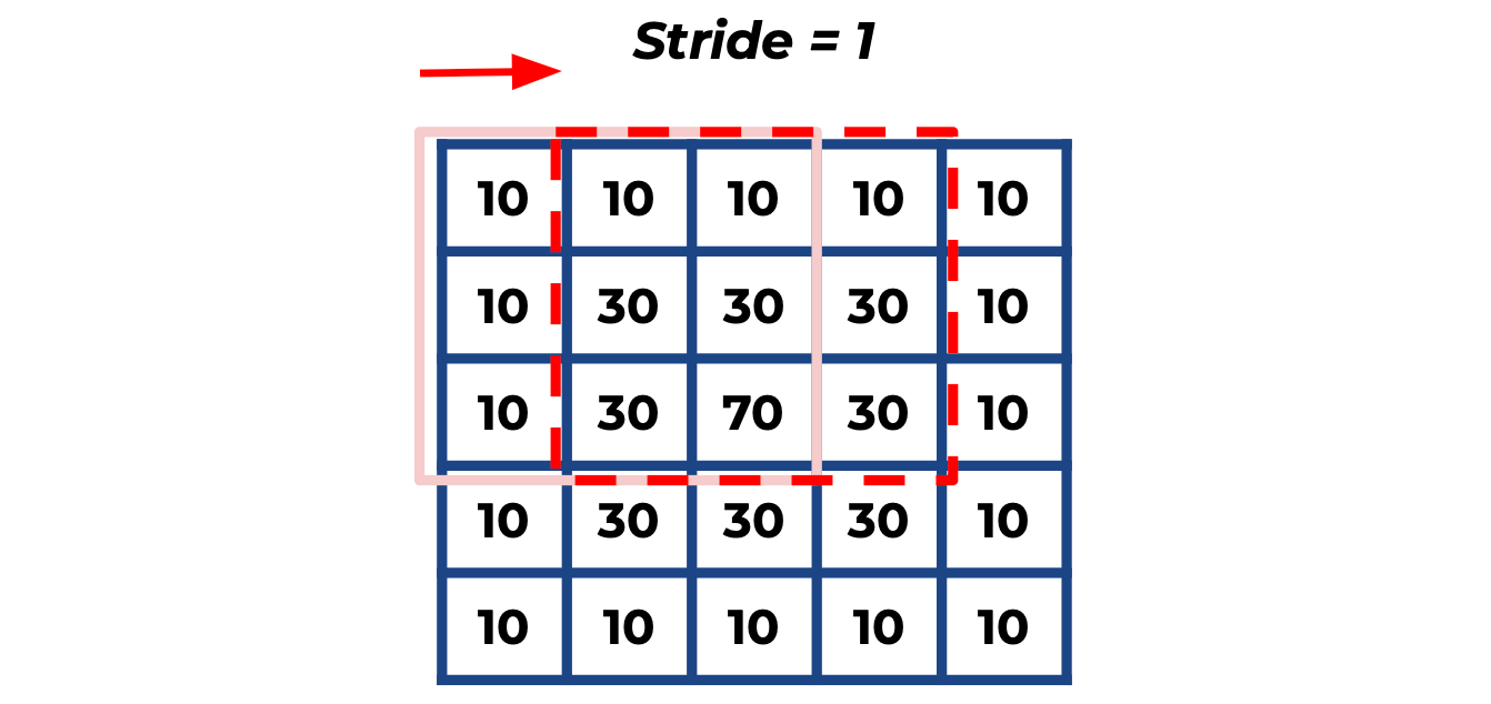
In the diagram below, we have a visual example of this process for the middle pixel of our input image.

Here we have an input grayscale image, which is 5×5 pixels, and a 3×3 kernel with all 1s that is causing a blurring effect (specifically a _box blur_).
The output for the middle pixel is calculated as follows:
[30*1 + 30*1 + 30*1] +
[30*1 + 70*1 + 30*1] +
[30*1 + 30*1 + 30*1]

= 30 + 30 + 30 + 30 + 70 + 30 + 30 + 30 + 30 = 310

pixel value = 310 / 9 ~ 34
This process is repeated by sliding the kernel and computing the convolution at each pixel. The corresponding output is referred to as a "feature map."
Below is the full result of applying the above kernel to the image.

Types of Kernel
Depending on the structure of a kernel, it will apply different effects to the input image. Below is a diagram of some commonly used kernels and their effect:

For machine learning and Computer Vision, one of the most useful kernels is the one that can detect edges. One example is the Sobel operator, which detects edges by measuring the gradient of intensity on either side of a pixel. So, if there is a big distinction in pixel values on either side of a pixel we are measuring, it's likely that there is an edge around that pixel.
The Sobel operator has two kernels, one for vertical gradients and the other for horizontal gradients:

I have a full article on the Sobel operator if you would like to learn more about it:
Convolutional Layers
Why?
You might be wondering why we need to know all this convolution rubbish. Why can't we use a fully connected neural network and flatten the pixels into a single dimension?
It works on the famous _MNIST dataset, but those are small images of 28×28 pixels. High-definition (HD) images have 1280×720 pixels. That's approximately 1,000,000 pixels, which is 1,000,000_ neurons in the input layer. Not to mention the millions of weights required for the hidden layers, rendering fully connected neural networks unsuitable for these images due to the dimensional complexity.
This is where we turn to CNNs and use the convolution operation and have partially connected layers. In other words, not all input neurons affect all output neurons. This greatly reduces the computational cost.
How Do Convolutional Layers Work?
We have seen how kernels (filters) extract information from an image. However, what if we allowed the machine or even a neural network to learn what kernels are the best to decipher what the image is?
The values in the kernels can be the weights and we can stack multiple kernel convolution operations together to form several convolutional layers, analogous to hidden layers in a fully connected neural network. Then, the neural network can adjust these weights inside the kernel through backpropagation, so the network can find the best kernels.
Neurons in subsequent layers are only connected to a handful of neurons in the previous layer, defined by the size of the kernel. This allows the first few layers to recognise low level features and build up the complexity as we propagate through the network. This hierarchical learning makes CNNs particularly effective for computer vision.
The diagram below visualises this process and the convolutional layers:

In the case of RGB color images, we would need to apply a separate kernel for each channel. So, in the RGB case, it would be three kernels for each red, green, and blue two-dimensional input.
Padding & Stride
For the convolutional layers to have the same height and width as the previous layer, we apply something called zero padding. Below is an example of this process for some images:

Padding keeps the dimensionality constant and also increases the sampling of the pixels on the perimeter. If we didn't pad the input image, then the edge pixels will only be computed once by the kernel leading to lost pixels and information.
In general, the output dimension is defined as:

- _H_in and W_in_ are the height and width of the original input image.
- _H_filter and W_filter_ are the height and width of the kernel or filter.
- _Padding_height and Padding_width_ are the amount of padding applied to the height and width of the input image.
- _Stride_height and Stride_width_ are the step sizes of the kernel along the height and width of the input image.
Stride is how many pixels we slide the kernel over the input image. By increasing the stride we reduce the computational cost but also increase the chance of losing information from the input.
Multiple Kernels
In practice, each convolutional layer will have multiple kernels and output one feature map per kernel. For example, if a convolution layer has 32 kernels, the output volume will have a depth of 32, with each slice corresponding to a feature map produced by each kernel. This allows the CNN to learn different aspects since each kernel learns to recognise different features of the input.
In the case of an RGB image, the output would be 96 feature maps deep due to 32 feature maps for each channel. The dimensionality can also get even larger. Satellite images have extra frequencies such as infrared.
Theory & Maths
The value of the neuron in each layer is:

- {i,j,l} is the three-dimensional coordinates of the neuron, where l is the number of channels. So, for RGB it would be three.
- Input_{i,j,l} is the value of the image at position {i,j,l}.
- Kernel_{i,_j,l}_ is the value of the kernel (or filter) at position {i,j,l}.
- Output_{k} is the output feature map for the k-th kernel.
- Bias_{k} is a single scalar value associated with the neuron for the k-th kernel. The same concept as in a fully connected neural network.
- ∑_{i,j,l} is the product of the input and kernel values are summed over all positions {i,j,l}.
- f is the activation function, typically ReLU applied to the summed value. The activation function is used to bring non-linearity into the CNN. See my previous article below for why this is important:
PyTorch Example
Below is an example of how you would implement two convolutional layers in PyTorch:
import torch
import torch.nn as nn
import torch.nn.functional as F

class CNN(nn.Module):
    def __init__(self):
        super(CNN, self).__init__()

        # Convolutional layer 1: 1 input channel, 5 kernels/filters, kernel size 3x3
        self.conv1 = nn.Conv2d(1, 5, 3)

        # Convolutional layer 2: 5 input channels, 10 kernels/filters, kernel size 3x3
        self.conv2 = nn.Conv2d(5, 10, 3)

        # An example of a fully connected layer after the convolutional layers
        # This example assumes an input image size of 32x32
        self.fc1 = nn.Linear(10 * 6 * 6, 120) # 6*6 from image dimension
        self.fc2 = nn.Linear(120, 84)
        self.fc3 = nn.Linear(84, 2) # Assuming binary classification
Summary & Further Thoughts
Convolutional layers work by stacking the outputs of applying a kernel to some input images. These kernels can identify things such as edges, but it's up to the CNN to learn the best kernel for the task. Stacking allows us to learn features of the image at a greater complexity at each layer, which will then later be passed into a regular fully connected neural network.
Another Thing!
I have a free newsletter, Dishing the Data, where I share weekly tips for becoming a better Data Scientist. There is no "fluff" or "clickbait," just pure actionable insights from a practicing Data Scientist.
