Essential Guide to Continuous Ranked Probability Score (CRPS) for Forecasting
If I asked you how to evaluate a regression problem, you would probably name quite a few evaluation metrics, such as MSE, MAE, RMSE, MAPE, etc. What these metrics have in common is that they focus on point predictions.
The situation changes a bit when we want to train our models to focus on predicting distributions instead of a single point. In that case, we need to use different metrics, which are not as commonly covered in Data Science blog posts.
Last time, I looked into quantile loss (a.k.a. pinball loss). This time, I will walk you through another metric used to evaluate probabilistic forecasts – the Continuous Ranked Probability Score (CRPS).
Here are a few definitions to get us started
The first concept is an easy one, but it is still important to make sure we are on the same page. Probabilistic forecasts provide a distribution of possible outcomes. For example, while point forecasts would predict tomorrow's temperature as exactly 23°C, a probabilistic model might predict a 70% chance the temperature will be between 20°C and 25°C.
The second definition will be a refresher from your stats class. The cumulative distribution function (CDF) is a function that tells us the Probability that a random variable takes on a value less than or equal to a particular value.
I hope that was not too bad! And this should be enough to get us started on CRPS. Let's dive into it!

The intuition behind CRPS
Before diving into the formula and maths, let's first develop an intuitive understanding. Since we have already discussed temperature predictions, let's continue using that example.
Random trivia: the CRPS metric was developed by a meteorologist and became popular in the context of probabilistic weather forecasting.
We know that we are not just interested in a point forecast, but we want to express the uncertainty in our predictions. Because, as we know all too well, the weather can be quite unpredictable.
In general, CRPS helps us measure how good our probabilistic predictions are by considering the entire range of possible outcomes. The metric compares our predicted probabilities with the actual outcome, resulting in a single score that shows how close the prediction was to reality.
For the sake of this example, let's assume we have the following predictions with associated probabilities:
- A 50% chance of the temperature being between 20°C and 23°C,
- A 30% chance of it being between 23°C and 25°C,
- And a 20% chance of it being between 25°C and 27°C.
Now, let's say that tomorrow the temperature turns out to be 24°C. Let's see how we would evaluate our forecast using CRPS.
First, we would use the forecasted probabilities to create a CDF, which shows the probability that the temperature will be less than or equal to any given value. It is important to note here that CRPS considers all possible values, not just the range indicated in our predictions.
The plot of the CDF in our case would look something like this:

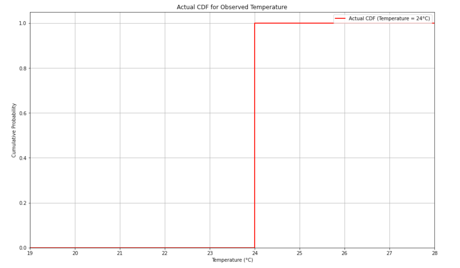
We already have the CDF of the predicted distribution. Then, we have to get the actual CDF. In this case, the actual CDF would be a step function at 24°C, since the observed temperature is a single value. The following plot illustrates this.
The last step is to calculate how close the predicted CDF is to the actual CDF. And this way we would arrive at the CRPS. To interpret the values, a lower CRPS score indicates that the predicted probabilities were closely aligned with the actual temperature.
To recap, you can think of CRPS as a tool that evaluates your forecast by assessing how well you captured the true uncertainty. Essentially, CRPS will penalize you if:
- You are too confident, for example, saying there's a 90% chance of 20–23°C, but the actual temperature is 25°C.
- You are too vague, for example, saying the temperature might be anywhere between 15°C and 30°C with equal probability.
The formula
Now that we have developed some intuition, let's look at the formula of CRPS:

Where F(x) is the CDF of the predicted distribution and 1() is an indicator function that equals 1 if the actual outcome y is less than or equal to x, and 0 otherwise.
As the formula contains an integral, this already hints that we are talking about an area between curves. Let's combine the two previous plots and visualize CRPS. For simpler plotting, I converted the predicted CDF from a step-wise one into a smooth one.
As you can see in the plot below, the CRPS is represented by the gray area between the two CDF curves. Mathematically, this is expressed by measuring the (squared) area enclosed between these two CDFs. Intuitively, we know that we want the distributions to be as similar as possible, so the area should be as small as possible.

In terms of the values, a lower CRPS indicates a better probabilistic forecast, suggesting that the predicted distribution is closer to the true outcome. Conversely, a higher CRPS indicates that the predicted distribution is less accurate. Unlike some other error metrics, CRPS is unbounded. Its value depends on the specific predictions and the scale of the target variable.
CRPS has another interesting property: when the predicted distribution is a degenerate distribution (e.g., a point forecast), CRPS reduces to the Mean Absolute Error (MAE). Without going into much detail, you can see the derivation below. For a point forecast y_hat, the CDF is degenerate and reduces to another indicator function.


Relation to quantile loss
Quantile loss focuses on the accuracy of predictions at specific quantiles, while CRPS generalizes this concept by evaluating the entire predicted CDF. In other words, we can think of CRPS as a continuous version of quantile loss across all possible quantiles.
As such, CRPS is a more comprehensive metric providing a single score that reflects the overall accuracy of the probabilistic forecast.
That said, we might prefer to use quantile loss when our goal is to predict specific quantiles – for example, when our model is trained specifically to predict the 10th and 90th percentiles of temperature.
On the other hand, we would likely opt for CRPS when our goal is to evaluate or optimize a model that outputs a full probabilistic forecast.
Wrapping up
In this article, we explored CRPS as a metric used to evaluate probabilistic forecasts. The main takeaways are:
- CRPS accounts for the entire probability distribution rather than just the mean or median forecast. As such, it provides a more comprehensive measure of accuracy that reflects uncertainty. This is because it not only evaluates how close you were to the actual value but also considers how well your forecast expressed the range of possible outcomes.
- CRPS penalizes forecasts that are too narrow (overconfident) or too wide (underconfident). As a result, it encourages well-calibrated forecasts.
- CRPS provides a single score that reflects the overall accuracy of the probabilistic forecast, making it easy to compare different models or forecasts. Therefore, it is often used to assess the relative accuracy of two probabilistic forecasting models.
As always, any constructive feedback is more than welcome. You can reach out to me on LinkedIn, Twitter, or in the comments.
Until next time
