Optimizing Pandas Code: The Impact of Operation Sequence

PYTHON PROGRAMMING

Pandas offer a fantastic framework to operate on dataframes. In data science, we work with small, big – and sometimes very big dataframes. While analyzing small ones can be blazingly fast, even a single operation on a big dataframe can take noticeable time.

In this article I will show that often you can make this time shorter by something that costs practically nothing: the order of operations on a dataframe.

---

Imagine the following dataframe:

import pandas as pd

n = 1_000_000
df = pd.DataFrame({
    letter: list(range(n))
    for letter in "abcdefghijklmnopqrstuwxyz"
})

With a million rows and 25 columns, it's big. Many operation on such a dataframe will be noticeable on current personal computers.

Imagine we want to filter the rows, in order to take those which follow the following condition: a < 50_000 and b > 3000 and select five columns: take_cols=['a', 'b', 'g', 'n', 'x']. We can do this in the following way:

subdf = df[take_cols]
subdf = subdf[subdf['a'] < 50_000]
subdf = subdf[subdf['b'] > 3000]

In this code, we take the required columns first, and then we perform the filtering of rows. We can achieve the same in a different order of the operations, first performing the filtering and then selecting the columns:

subdf = df[df['a'] < 50_000]
subdf = subdf[subdf['b'] > 3000]
subdf = subdf[take_cols]

We can achieve the very same result via chaining Pandas operations. The corresponding pipes of commands are as follows:

# first take columns then filter rows
df.filter(take_cols).query(query)

# first filter rows then take columns
df.query(query).filter(take_cols)

Since df is big, the four versions will probably differ in performance. Which will be the fastest and which will be the slowest?

Benchmarks

Let's Benchmark this operations. We will use the timeit module:

Benchmarking Python code with timeit

or rather its version available in the IPython shell.

These are our benchmarks:

In the following section, we'll analyze the results of the benchmarks, and then we'll interpret these results.

Results

Bracketing: select columns, then filter rows (16.5 ms)

subdf = df[take_cols]
subdf = subdf[subdf['a'] < 50_000]
subdf = subdf[subdf['b'] > 3000]

In this code, we used typical Pandas code based on brackets, Boolean indexing, and assignments. To achieve the expected result, we used three lines in the following order: we started off by selecting a subset of columns and then applied the two filtering conditions sequentially.

Among the four approaches, this one was relatively fast – but not the fastest. Selecting columns first reduces the width of the df dataframe, but note that it is not primarily the width that makes the dataframe so large. It's the number of rows. Look¹:

In [7]: n_of_elements = lambda d: d.shape[0]*d.shape[1]

In [8]: n_of_elements(df)
Out[8]: 25000000

In [9]: n_of_elements(df.filter(take_cols))
Out[9]: 5000000

In  [10]: n_of_elements(df.query(query))
Out [10]: 1174975

As we can see, when we remove the columns first (df.filter(take_cols)), we get a dataframe of 5 million elements, while filtering the rows first (df.query(query)) gives a dataframe of just over a million elements, which is more than four times smaller.

It's no wonder that removing the unnecessary columns first makes the operation slower than removing the unnecessary rows first – as shown in the next section.

Bracketing: filter rows, then select columns (10.7 ms)

subdf = df[df['a'] < 50_000]
subdf = subdf[subdf['b'] > 3000]
subdf = subdf[take_cols]

This code also uses typical Pandas code based on brackets, Boolean indexing, and assignments, but this time, rows are filtered first in order to reduce the size of the dataframe; then the selected columns are taken.

This is clearly the fastest approach among the four tested. The efficiency gains are due to the reduction in the dataframe size early in the process, thereby providing a smaller dataset to process in the subsequent steps.

In this approach and the previous one, we used truly vectorized Pandas code, meaning that it used direct Boolean indexing. Theoretically, it is vectorized operations that offer the most performant Pandas code – and we can see it. The difference between the two versions results from what we've just analyzed: the fact that you should use this operation first which will reduce the dataframe's size the most.

Pipes: select columns, then filter rows (26.0 ms)

df.filter(take_cols).query(query)

This code uses chained Pandas operations. It starts by filtering rows, and then it takes the required columns.

Note that the .query() method of Pandas dataframes doesn't use vectorized operations in the traditional Pandas/Numpy meaning. Instead, it uses the [numexpr](https://pypi.org/project/numexpr/) Python package. While theoretically, as the documentation says,

NumExpr is a fast numerical expression evaluator for NumPy.

we see that in our experiment it was slower than vectorized operations based on Boolean indexing.

Returning to our benchmarks, it is noticeably the slowest code among the ones observed. There are two reasons for this: chaining Pandas operations is slower than vectorizing them, and as we have just discussed, reducing the number of columns first is less efficient for this dataset than filtering the rows first. Although the .filter() method reduces the dataframe's size, this reduction is over four times smaller than that achieved after reducing the number of rows via .query().

Pipes: filter rows, then select columns (17.3 ms)

df.query(query).filter(take_cols)

We can consider this code an improved version of the previous one. We know already that we should first get rid of the unnecessary rows, and only then select the required columns – and this code does so via chained Pandas operations.

While this method is more efficient than the previous one (a pipe that selects columns and then applies .query()), it still doesn't match the Performance of the corresponding vectorized code. It's more or less similarly performant as the vectorized code in the less effective order.

Interpretation

The benchmarks led to the following observations, which emphasize the role of vectorized operations and operation order:

• Vectorized row filtering first: The results highlight the importance of minimizing the dataframe size early in the workflow. By reducing the number of rows first, subsequent operations – in our case, column selection – operate on a smaller dataset, which improves speed.
• Efficiency of column selection: Starting the workflow by selecting columns does reduce memory usage by narrowing the dataframe – which leads to shorter execution. This reduction in time, however, is smaller than that achieved by starting by filtering rows. Thus, this version is not optimized for processing speed.
• Chaining operations: While this is not the topic of this article, we did observe that chaining Pandas operations is less efficient than vectoring them. The execution times for pipes (17.3 ms and 26 ms) illustrate this phenomenon, as they are visible slower than the corresponding vectorized operations (10.7 ms and 16.5 ms, respectively).

Do remember, however, that this interpretation is not general; it refers to our benchmarks and the particular scenario we analyzed.

I will leave you with an exercise: Does it matter which row filtering will you apply first, a < 50_000 or b > 3000?

More columns than rows

Above, we worked with a dataframe that had more rows than columns, but what if the situation is opposite, that is, we work with a dataframe that has many columns and much fewer rows?

From what we learned above, it follows that our main criterion behind choosing the order of operations is the size of the resulting dataframe. So, let's analyze the following scenario:

Do you see this? This is 718 µs versus 121 ms, so the first approach (select columns first) is significantly faster— almost… 170 times faster! The reason is just like before – the size of the dataframe after the first operation. This time the difference is huge:

The second operations also operate on dataframes of very different sizes:

Interestingly, chained Pandas operations work very inefficiently for such dataframes:

Note that we tool the columns first, and still this pipe required only three times less time than the slow operation above. I did try benchmarking (for -n 1) the corresponding pipe with the reversed order of operations, but after some three hours, I killed the benchmark:

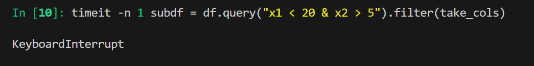
Clearly chained operations do not work well for dataframes with so many columns (here, a million columns).

Conclusions

Our experiment illustrates an important principle of data manipulation in Pandas: reducing the dataset size as soon as possible, particularly through vectorized row filtering operations, can significantly improve performance.

While this recommendation doesn't come as a surprise but looks rather quite obvious, I must admit that in the past, I sometimes failed to follow it. From now on, I will for sure remember to think about the sequence of Pandas operations.

Certainly, when you analyze a small dataframe in an interactive session, you can ignore performance differences and use whatever code you prefer. But in production code, the sequence of operations can make quite a difference – whether analyzing a large dataframe or many small ones.

In our first example, applying row filtering before column selection emerged as the more efficient strategy than the opposite order. It's not a general observation, however – it depends on the dataframe.

We used the number of elements in a dataframe as the main criterion, but do note that it's not enough – it also matters whether the dataframe is long or wide. We analyzed two dataframes of the same number of elements, and we saw great differences in performance.

Thus, if performance matters, you should analyze each dataframe individually and choose the order of operations with care, taking its shape and size into account. This insight is invaluable for optimizing pandas workflows, especially when dealing with large datasets.

Let's summarize. Our benchmarks lead to the following key insights into implementing Pandas operations:

• Vectorizing Pandas operations leads to more performant code than chaining Pandas operations.
• Generally, to implement performant code that incorporates several Pandas operations, follow the shape and size of the dataframe in subsequent steps: start with operations that will most significantly reduce the size of the dataframe, and end with those which reduce this to the least extent.
• When performance matters, optimize each piece of code individually, taking into account the shape and size of the dataframe.

If performance matters, you should analyze each dataframe individually and choose the order of operations with care, taking its shape and size into account.

Footnotes

¹ In this code, I defined a named function using the following lambda definition:

Python">In [7]: n_of_elements = lambda d: d.shape[0]*d.shape[1]

Yes, I did use a named lambda definition. As I explain here:

Should You Define Named Python Functions Using lambda?

theoretically you should not use named lambdas, but here:

Data Analysis with Named Lambda Functions

I show an exception to this rule: data analysis code that is not going to be saved or distributed.

Ironically, I did distribute this very code, but to make a point rather to make myself a rebel.

Tags: Benchmark Data Science Pandas Performance Python

Comment